Do Gaussian Processes scale well with dimension?
March 16, 2024
This blogpost assumes you’re already familiarized with the basics of Gaussian Processes. Check my previous blogpost for an introduction.
[Update] Here’s a link to the (very unpolished) code I used for the experiments in this blogpost.
It’s folk knowledge that Gaussian Processes (GPs) don’t scale well with the dimensionality of their inputs. Some people even claim that, if the problem goes beyond 20 input dimensions, then GPs fail to do regression well.1
The main hypothesis is that GPs fail because of the curse of dimensionality: since the usual (stationary) kernels base their computation of correlation on distance, there’s less signal in higher dimensions because distances become meaningless. Other reasons why GPs might fail could be having difficult loss landscapes or numerical instabilities.2
These hypotheses might be misguided. Last month, Carl Hvarfner, Erik Orm Hellsten and Luigi Nardi released a paper called Vanilla Bayesian Optimization Performs Great in High Dimensions, in which they explain the main reasons why GPs fail in high dimensions, disputing and disproving this folk knowledge.
In this blogpost I explore the failures of GPs to fit in high dimensions using the simplest example I could imagine, following what Hvarfner et al. propose in their recent paper.3 I only assume that you’re familiar with my previous blogpost on GPs and Bayesian Optimization.
Vanilla GPs fail to fit to simple functions #
A really simple function #
Consider the shifted sphere function \(f_{\bm{r}}:\mathbb{R}^D\to\mathbb{R}\) given by \[f_{\bm{r}}(\bm{x}) = \sum_{i=1}^D (x_i - r_i)^2,\] where \(\bm{r}\) is a random offset. This function is extremely simple. In 2 dimensions it’s a parabola, in 3 it’s a paraboloid, and so on. It’s a second-degree polynomial on its inputs \(\bm{x} = (x_1, \dots, x_D)\) , and it is as smooth as functions come.
Fitting a GP to it #
Consider the most vanilla GP: an exact model with an RBF kernel
class ExactGPModel(gpytorch.models.ExactGP):
    def __init__(self, train_x, train_y, likelihood):
        super(ExactGPModel, self).__init__(train_x, train_y, likelihood)
        _, n_dimensions = train_x.shape

        self.mean_module = gpytorch.means.ConstantMean()
        self.covar_module = gpytorch.kernels.ScaleKernel(
            gpytorch.kernels.RBFKernel(ard_num_dims=n_dimensions)
        )

    def forward(self, x):
        mean_x = self.mean_module(x)
        covar_x = self.covar_module(x)
        return gpytorch.distributions.MultivariateNormal(mean_x, covar_x)
We should expect it to fit our shifted sphere function quite easily, even in high dimensions. Let me show you how and when it fails.
For our training set, we sample \(N\) points from a unit Gaussian in \(D\) dimensions and add a little bit of random noise: \[\begin{array}{ll} \bm{x}_n \sim \mathcal{N}(\bm{0}, \bm{I}_D)&\text{(data dist.)}\\[0.2cm] y_n = f_{\bm{r}}(\bm{x}_n) + \epsilon,\epsilon \sim \mathcal{N}(0, 0.25)&\text{(noisy output)}. \end{array}\]
And indeed, in the 1D case we get a pretty good fit:4
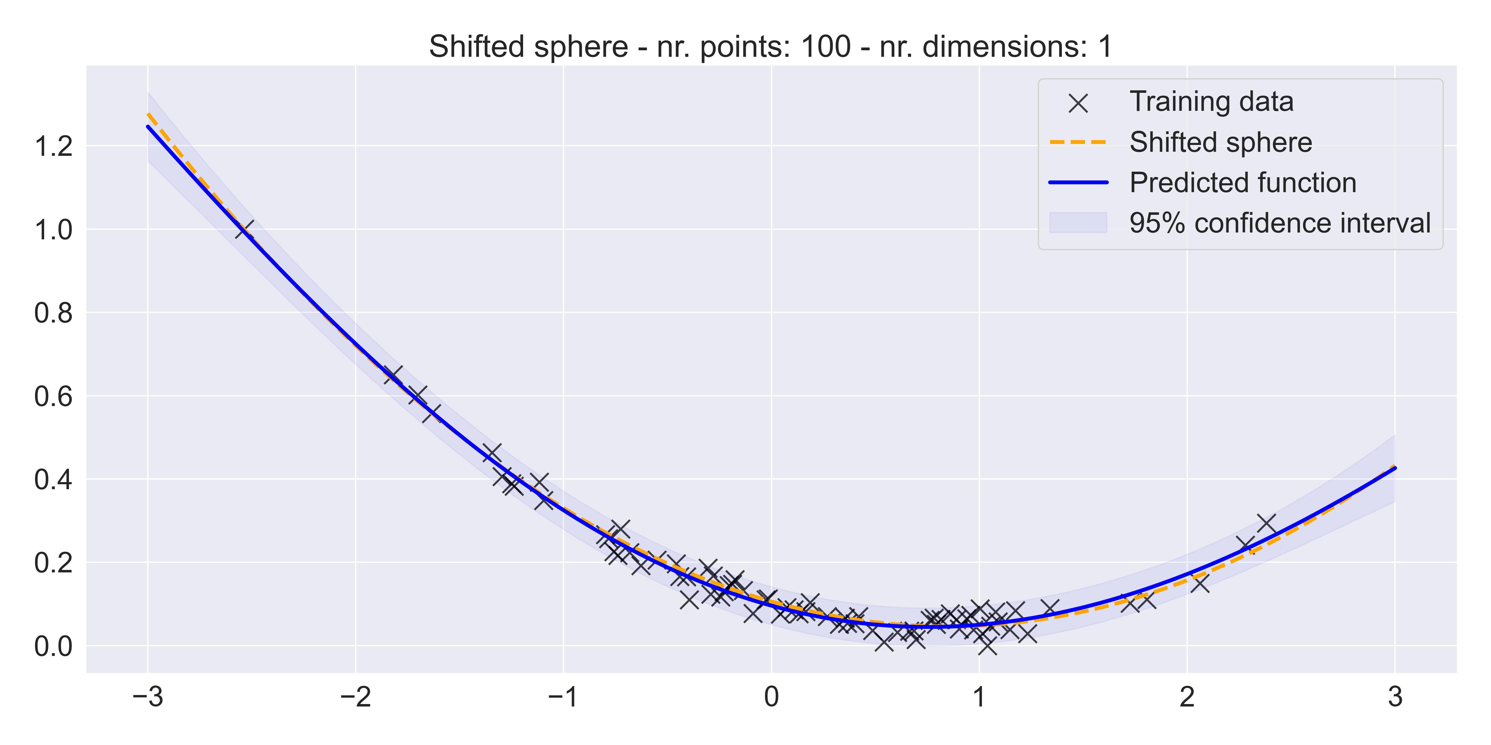
Fitting a vanilla GP to a shifted sphere
We can also quantify the quality of the fit by plotting the mean predicted values against the actual values for a small test set of 50 points, sampled from the same distribution and corrupted in the same way. This plot is useful, because it can be computed regardless of the input dimension:
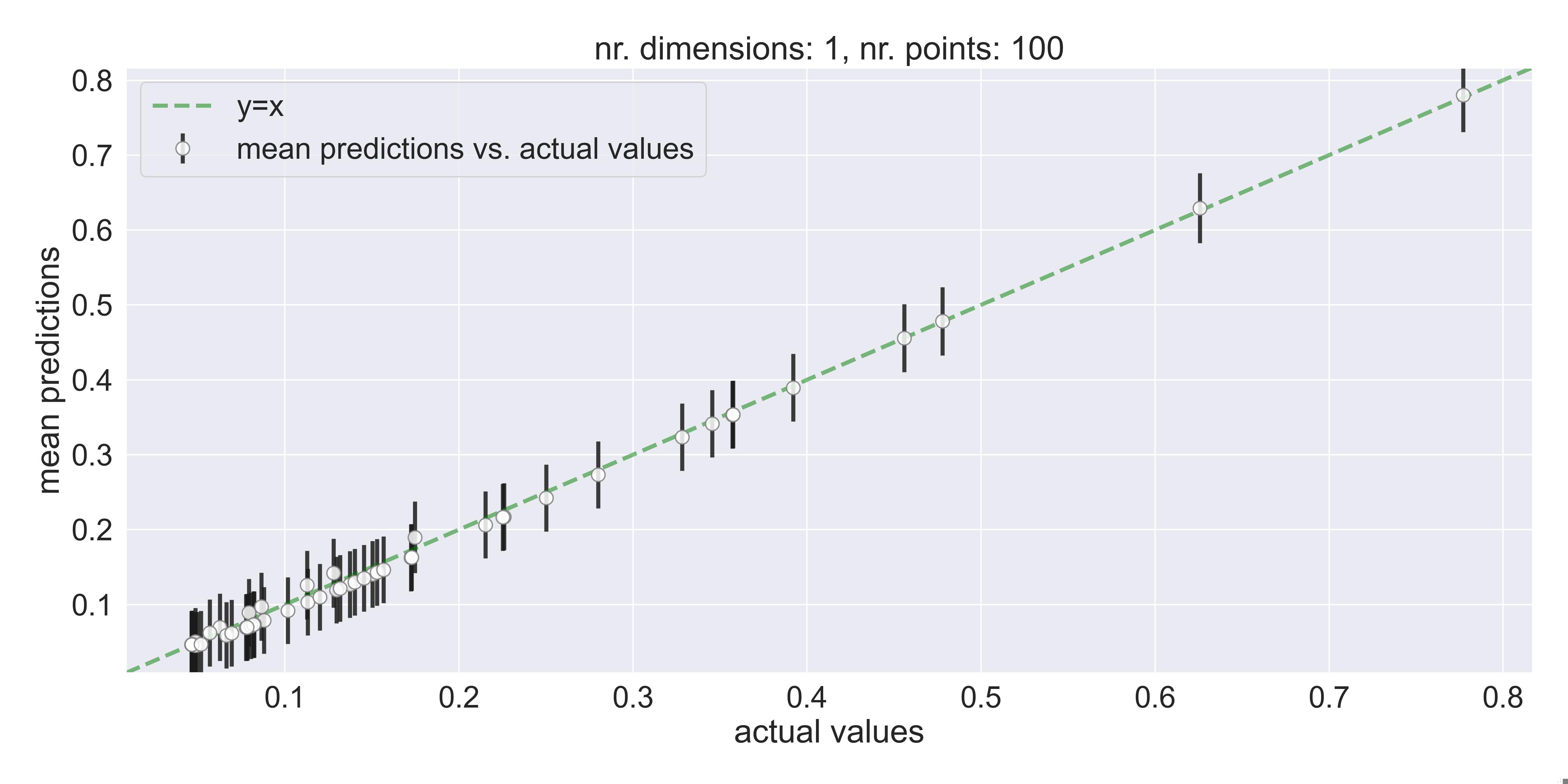
A good fit - predictions and actual values are highly correlated
What happens if we go to higher dimensions? #
Let’s try to fit this exact same function, but with \(D=64\) . Since we can’t visualize \(\mathbb{R}^{64+1}\) space, we can only rely on these second plots I showed you, the ones that compare predictions to actual values… Immediately, we can see that vanilla GP fails and defaults to predicting just the mean:
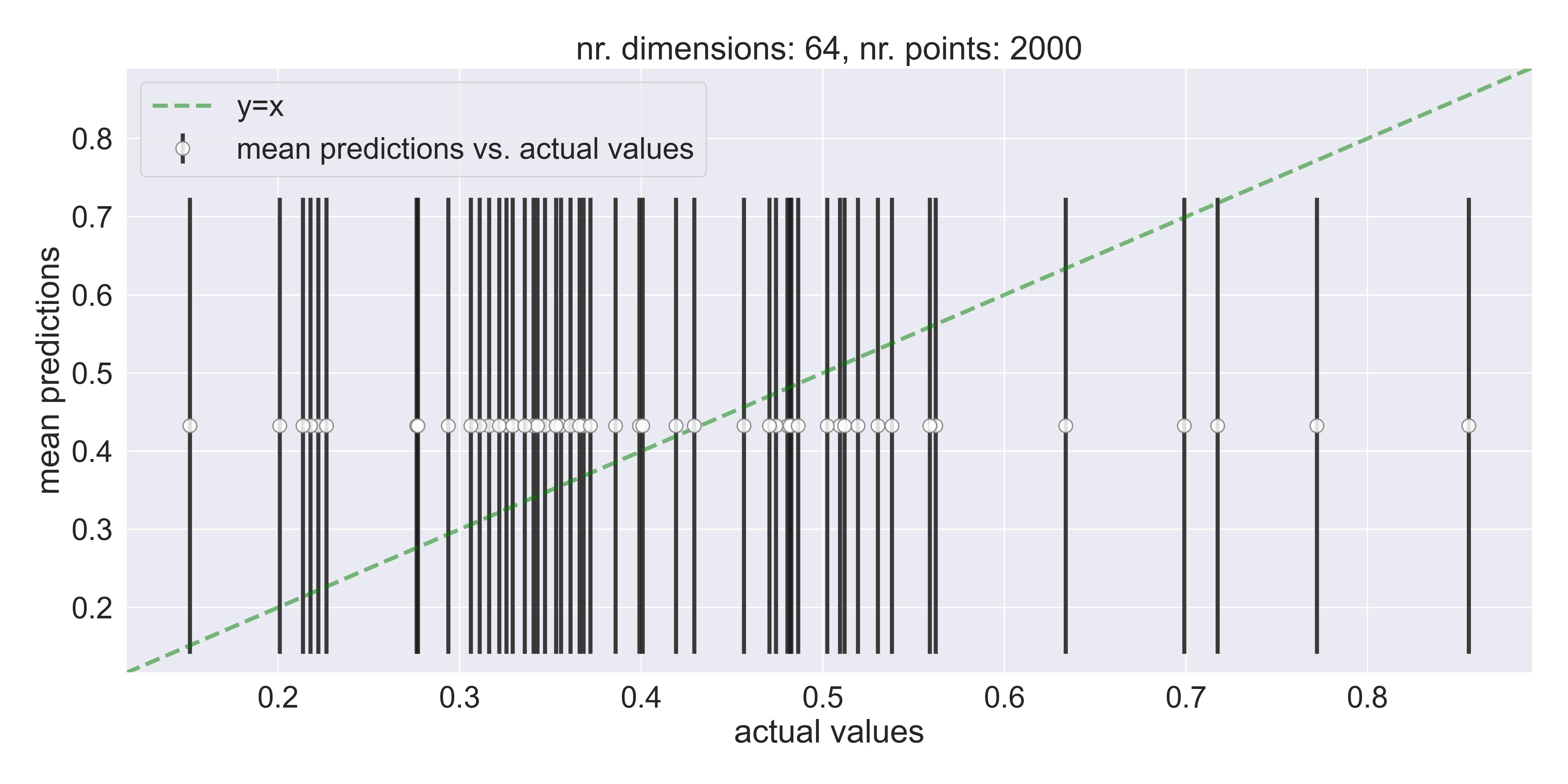
A bad fit - predictions default to the mean on 64 dimensions, even when using 2000 training points
The model didn’t learn a thing. It’s defaulting to a certain mean prediction. Let me try to find exactly when GPs start to fail. Folk knowldege says it’s around 20 dimensions, but if we sweep for several values of \(N\) and \(D\) , we get the following table:
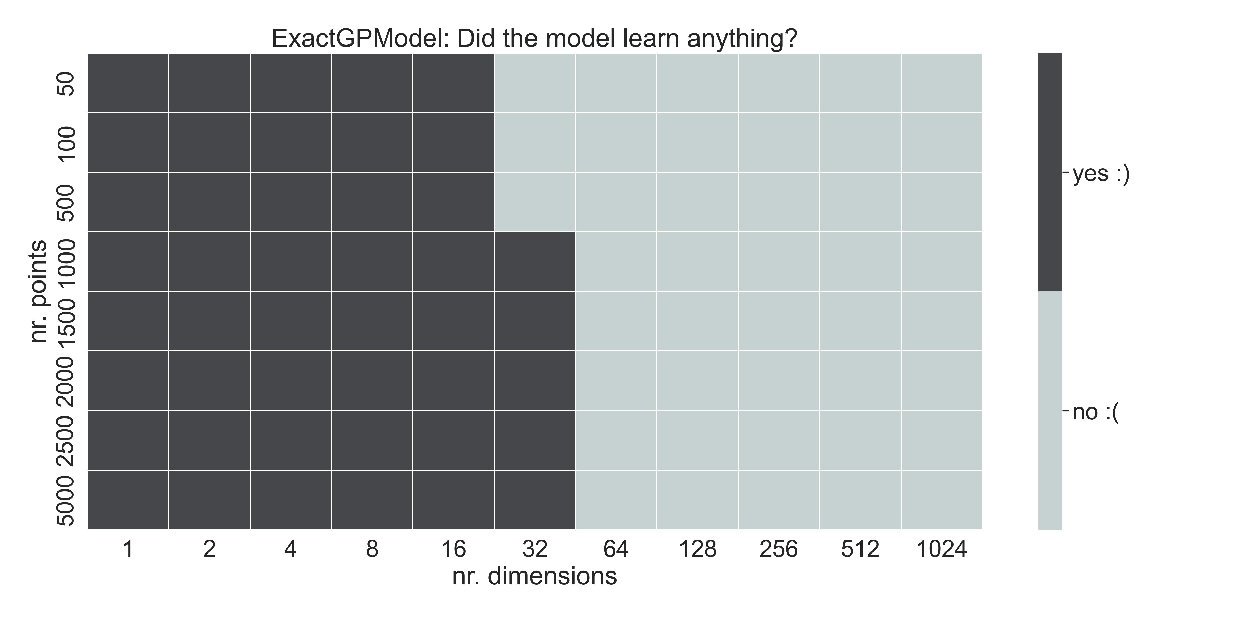
Table - nr. of training points & input dimension, and whether the model learned anything
where yes :) means that the model learned something, and didn’t default to the mean. The breaking point for this function in particular seems to be around 32 dimensions, and we notice that the number of training points is of course important.
Why?! #
Why are GPs failing to fit even a simple function like a high-dimensional paraboloid? As I said in the introduction, the community argues that this is a failure of stationary kernels’ use of distance for correlation. In the next section I talk a little bit about kernels and about the curse of dimensionality.
The curse of dimensionality and kernel methods #
Measuring correlation using kernels #
Recall that GPs assume the following: given a function \(f\colon\mathbb{R}^D\to\mathbb{R}\) and two inputs \(\bm{x}, \bm{x}'\in\mathbb{R}^D\) , then \[\text{cov}(f(\bm{x}), f(\bm{x}')) = k(\bm{x}, \bm{x}')\] where \(k\colon\mathbb{R}^D\times\mathbb{R}^D\to\mathbb{R}\) is a kernel function (i.e. symmetric positive-definite).
In other words, we make statements about how correlated two function evaluations are (the left side of the equation) using kernels as a proxy (the right side).
A large family of these kernels (called stationary) only depend on the distance between inputs \((x_i - x_i')^2\) , such as the Radial Basis Function (RBF):
\[k_{\text{RBF}}(\bm{x}, \bm{x}';\,\sigma, \Theta) = \sigma\exp\left(-\frac{1}{2}(\bm{x}-\bm{x}')^\top\Theta^{-2} (\bm{x}-\bm{x}')\right),\] where \(\sigma>0\) is an output scale, and \(\Theta\) is a diagonal matrix with lengthscales \(\lambda_i, i=1,\dots,D\) .
The curse of dimensionality #
Put shortly, the curse of dimensionality says that distances start to become meaningless in higher dimensions, and that space becomes more and more sparse.
We can actually quantify this with a simple experiment: consider a collection of points \(\{x_n\}_{n=1}^N\) in \([0,1]^D\subseteq\mathbb{R}^D\) , sampled uniformly at random in the unit cube. What can we say about the distribution of the pair-wise distances?
Consider the following Python script for randomly sampling a collection of points and computing their pairwise distance (using jax for speed):
import numpy as np
import jax
import jax.numpy as jnp

@jax.jit
def pairwise_distances(x):
    # Using the identity \|x - y\|^2 = \|x\|^2 + \|y\|^2 - 2 x^T y
    distances = (
        jnp.sum(x**2, axis=1)[:, None] - 2 * x @ x.T + jnp.sum(x**2, axis=1)[None, :]
    )

    return distances


def compute_distribution_of_distances(
    n_points: int,
    n_dimensions: int,
):
    seed = np.random.randint(0, 10000)
    key = jax.random.PRNGKey(seed)

    # Warm-up for the JIT
    x = jax.random.uniform(key, (2, n_dimensions))
    distances = pairwise_distances(x)

    # Sampling from the unit cube and computing
    # the pairwise distances
    x = jax.random.normal(key, (n_points, n_dimensions))
    distances = pairwise_distances(x)

    # Keeping only the upper triangular part
    # of the distance matrix
    distances = jnp.triu(distances, k=1)

    return distances[distances > 0.0]


if __name__ == "__main__":
    N_POINTS = 1_000
    n_dimensions = [2**exp_ for exp_ in range(1, 8)]

    arrays = {}
    for n_dimensions_ in n_dimensions:
        distances = compute_distribution_of_distances(N_POINTS, n_dimensions_)
        arrays[n_dimensions_] = distances
Visualizing these distances renders this plot, where we color by different dimensions (from 2 ** 0 to 2 ** 7):
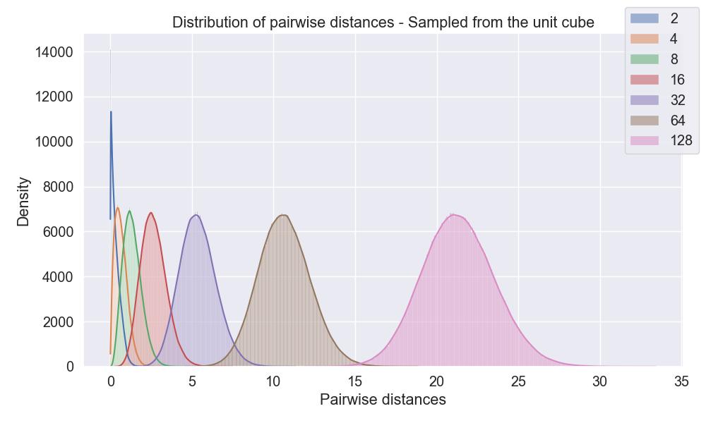
Notice how the average distance between randomly sampled points starts to grow, even if we restrict ourselves to the unit square.
Lengthscales, lengthscales, lengthscales #
Our stationary kernels should reflect this change in distance. By including lengthscales, our computation of correlation is actually mediated by hyperparameters that we tune during training. Lengthscales govern the “zone of influence” of a given training point: large values allow GPs to have higher correlation further away, and lower lengthscales mean that the zone of influence of a given training point is small, distance-wise. Fig. 2 of Hvarfner et al. 2024 exemplifies this.
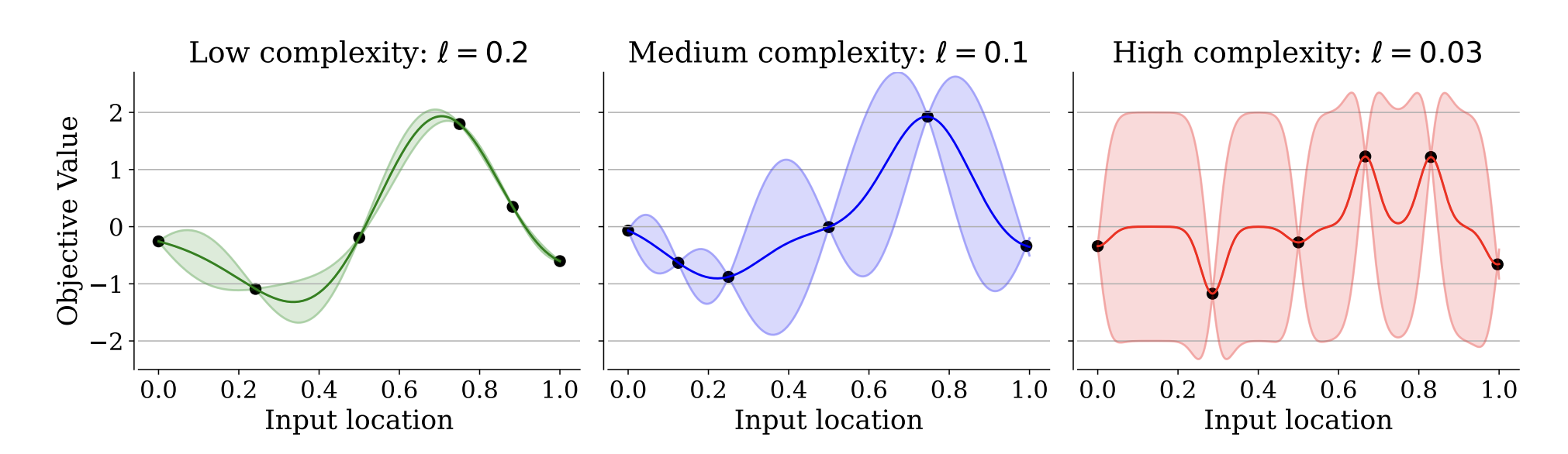
The impact of lengthscales on Gaussian Process regression. (Image source: Fig. 2 of Hvarfner et al. 2024)
How are the lengthscales looking in our simple examples? For the good fit we showed (the one in 1D, with 100 training points), the learned lengthscale is of around 3.64. In the 64D case, all lengthscales (which are supposed to be different) collapse to 0.693 during training.
A simple fix: Imposing larger lengthscales #
Hvarfner et al.’s insight is this: we should be encouraging larger lengthscales. They phrase it in the language of model complexity, saying that the functions we might be fitting are not as complex as we think. There’s a mismatch, according to them, between the assumed complexity and the actual complexity of the functions we’re fitting.
Larger lengthscales would allow the kernel to assume correlation between points that are further away, mitigating the curse of dimensionality.
How do we encourage larger lengthscales during training? The answer is easy: add a regularization to the loss.
MAP vs. MLE estimates #
In the previous blogpost, I vaguely stated that kernel hyperparameters can be trained by maximizing the log-marginal likelihood w.r.t. the training points. Being a little bit more explicit, the function we are trying to maximize is this:
\[\log p(\mathbf{y}|\bm{x}_1,\dots,\bm{x}_N, \theta) = -\frac{1}{2}\mathbf{y}^T(K + \sigma_n^2I)^{-1}\mathbf{y} - \frac{1}{2}\log\det(K + \sigma_n^2I) - \frac{n}{2}\log(2\pi),\] where \(\bm{y}\) are the noisy observations, \(K=[k(\bm{x}_i, \bm{x}_j)]\) is the Gram matrix, \(\sigma_n > 0\) is a noise scale, and \(\theta\) represents all kernel hyperparameters, including of course the lengthscales and \(\sigma_n\) .
Maximizing this quantity w.r.t. \(\theta\) results in what is called the Maximum Likelihood Estimate, or MLE.
To encourage larger lengthscales, we can add a prior distribution for them, and try to maximize the a posteriori distribution \(p(\theta|\bm{y}, \bm{x}_1,\dots,\bm{x}_N)\) , which is proportional to the product of the likelihood \(p(\bm{y}| \bm{x}_1,\dots,\bm{x}_N, \theta)\) and the prior \(p(\theta)\) . The new function we would try to maximize would then be:
\[\underbrace{-\frac{1}{2}\mathbf{y}^T(K + \sigma_n^2I)^{-1}\mathbf{y} - \frac{1}{2}\log\det(K + \sigma_n^2I) - \frac{n}{2}\log(2\pi)}_{\text{The usual marginal log-likelihood}} + \underbrace{\log p(\theta)}_{\text{Regularizer}}.\]Maximizing this renders the Maximum a posteriori (MAP) estimate. Tools like GPyTorch allow us to add these regularizers easily using keyword arguments of kernels.
To summarize, saying “I’m using MAP estimation” is just a fancy way of saying “I’m adding a term to my loss to encourage a certain behavior in my kernel hyperparameters”. Phrasing this in a probabilistic language is useful, because we can be more precise about which values we’d like our lengthscales to take by thinking of them as distributions.
Some priors for likelihoods #
By default, gpytorch considers no prior on the lengthscales. botorch’s default SingleTaskGP has a
\(\lambda_i \sim \text{Gamma}(3, 6)\)
prior, which has an average value of
\(\mathbb{E}[\lambda_i] = 1/2\)
and a standard deviation of around
\(\sigma_{\lambda_i} = 3/6^2 \approx 0.083\)
. Here’s the density of this prior:5
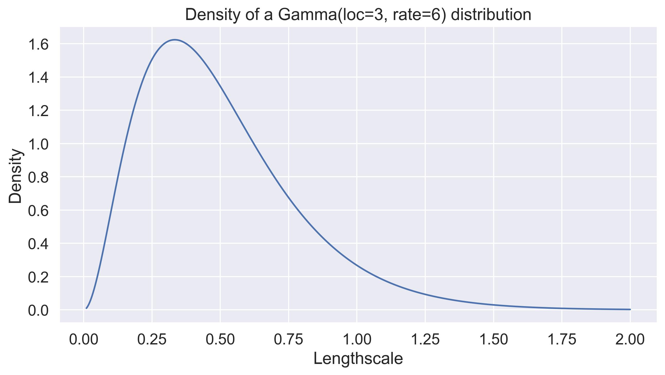
Default lengthscale prior in botorch. It places priority on small lengthscales and doesn't scale with D.
Notice how this places a huge weight on small lengthscales, and is entiery independent of the dimensionality of the input space. As our plot above shows, for dimensionalities above 64, the expected distances between randomly sampled points is already above 20.
Hvarfner et al. propose a simple prior that does depend on the dimension of the input space: \[p(\lambda_i) = \text{logNormal}(\mu_0 + \log(D)/2, \sigma_0),\] where \(\mu_0\) and \(\sigma_0 > 0\) are parameters that could be learned as well.6 Let’s visualize this prior for different dimensions and for a fixed value of these hyperparameters:
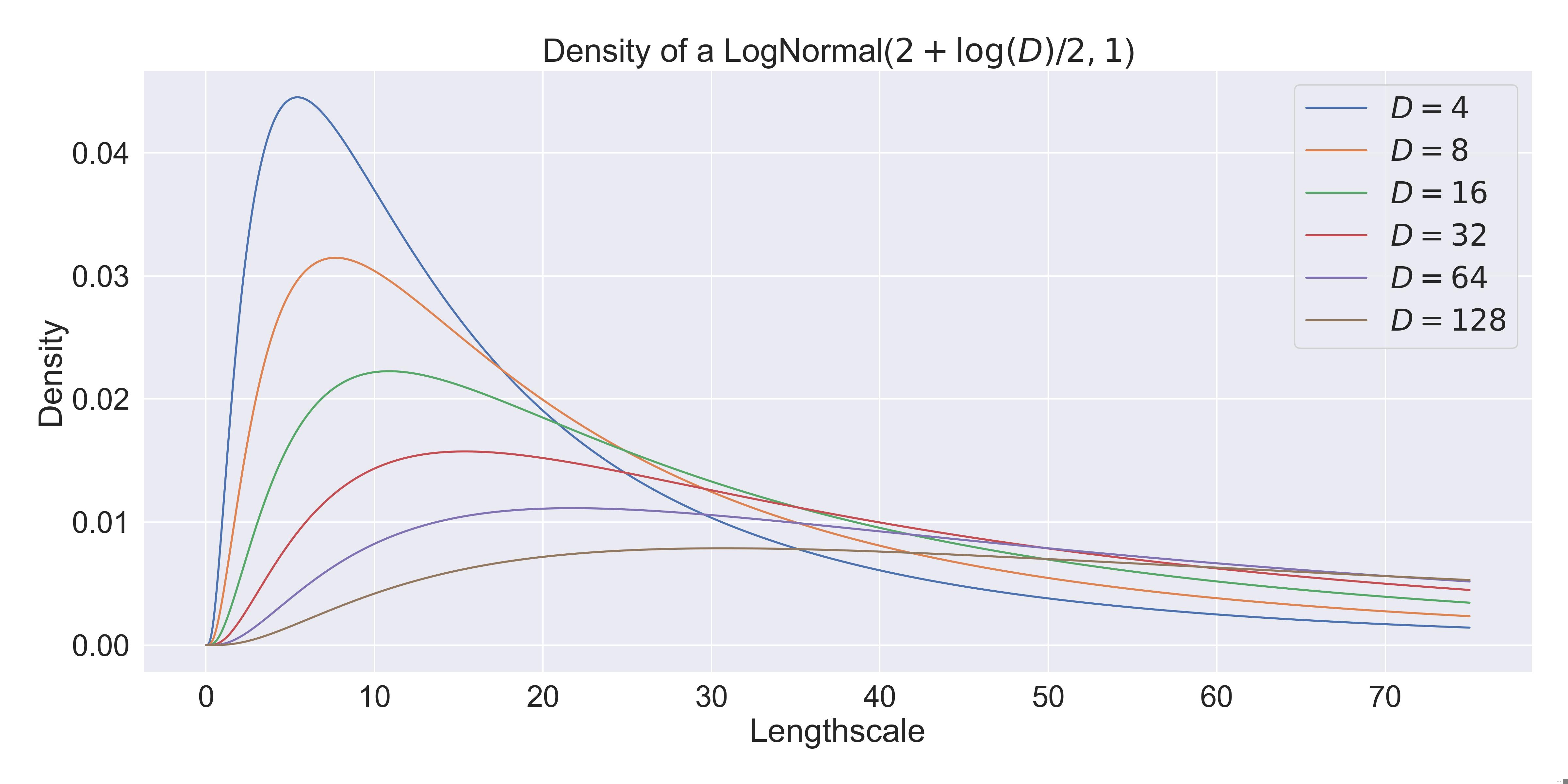
Density proposed by Hvarfner et al. - Now we're scaling with the dimension.
Applying this fix #
Applying this fix is as simple as adding a single line to our torch models:
class ExactGPModelWithLogNormalPrior(gpytorch.models.ExactGP):
    def __init__(self, train_x, train_y, likelihood):
        super(ExactGPModelWithLogNormalPrior, self).__init__(
            train_x, train_y, likelihood
        )
        _, n_dimensions = train_x.shape

        # With a little elbow grease, these
        # could be trainable parameters as well.
        mu_0 = 0.0
        sigma_0 = 1.0

        self.mean_module = gpytorch.means.ConstantMean()
        self.covar_module = gpytorch.kernels.ScaleKernel(
            gpytorch.kernels.RBFKernel(
                ard_num_dims=n_dimensions,
                # THE ONLY CHANGE IS THE FOLLOWING LINE:
                lengthscale_prior=gpytorch.priors.LogNormalPrior(
                    mu_0 + np.log(n_dimensions) / 2, sigma_0
                ),
            )
        )
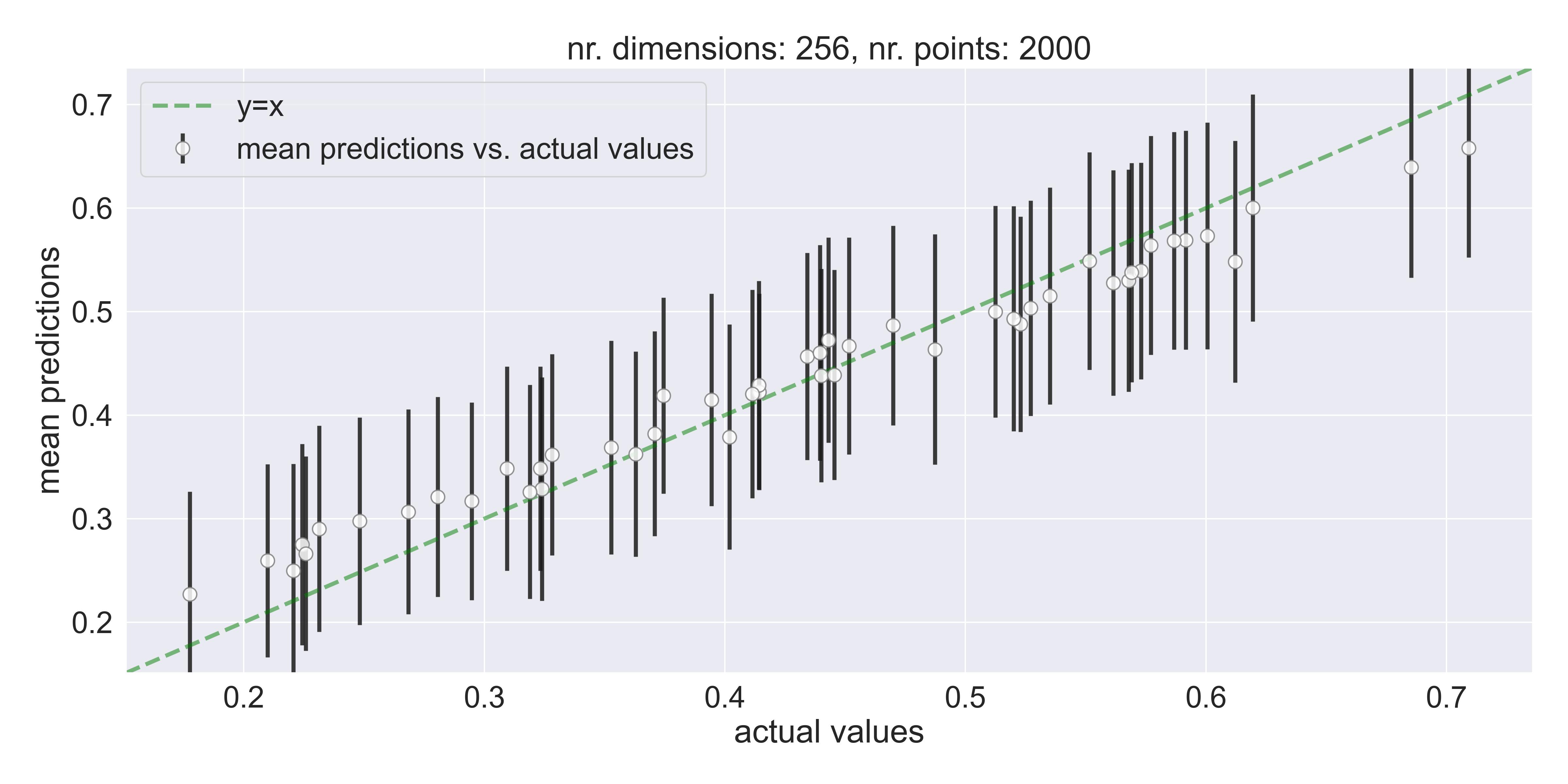
Adding this prior has a dramatic impact on whether the model is able to fit above 32 dimensions in the toy example discussed previously. Here’re the model’s predictions in, say, 256 dimensions:
A good fit in high dimensions - Adding a scaling to the prior allows exact GPs to fit high dimensional data.
We can compute the same table we showed for ExactGPModel, but for this one:
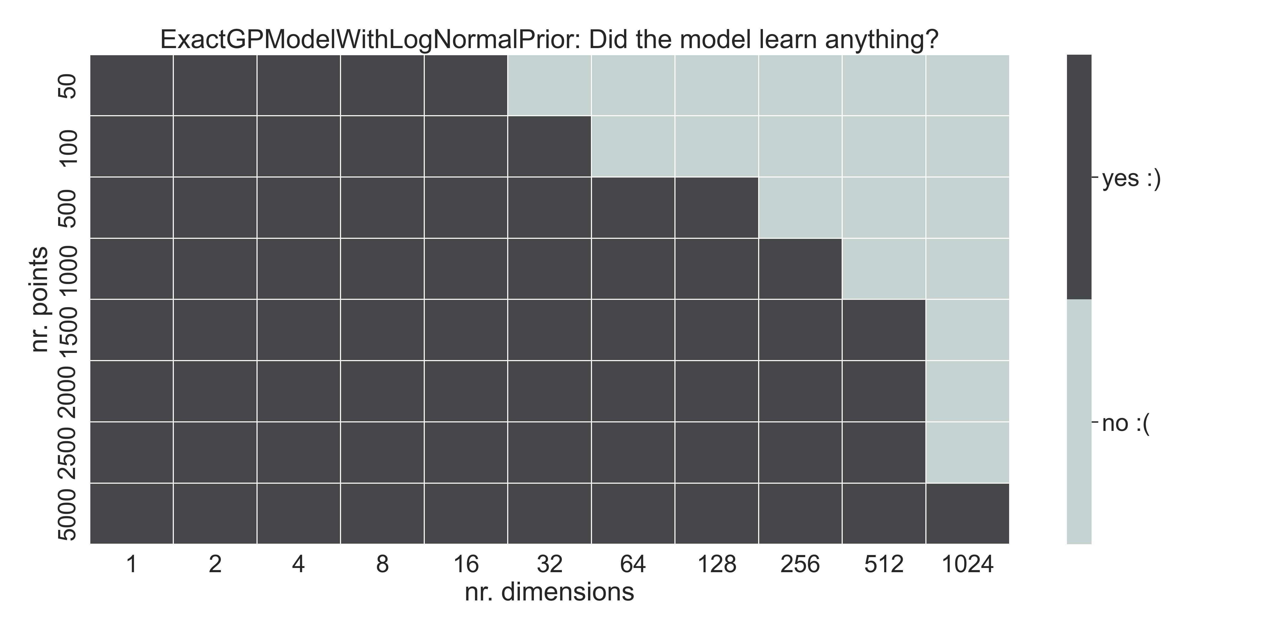
Same table as before - With the given prior, the model learns up to 1024 dimensions with enough training data.
Now we can fit up to 512 dimensions easily! With enough data, we might be able to fit 1024 dimensions as well.
Conclusion #
Recent research seems to show that vanilla Gaussian Processes are actually capable of going beyond the folk 20-ish dimensions limit. In this blogpost I explored the toy-est of toy examples, and showed you how even a simple polynomial function can’t be fitted by vanilla Gaussian Process Regression in high dimensions.
As Hvarfner et al. recognize, this might be a problem with the lengthscales and the assumed complexity of the functions we’re fitting. Incorporating a prior on the lengthscales, as they propose, allows exact GP regression to fit our higher dimensional toy problem.
I discussed these results with Joachim, a colleague, and he asked a natural question: what’s stopping us, then, from having GPs fit in \(D>10000\) dimensions? Are there any more inherent limitations of exact GP inference (besides, of course, training dataset sizes)?
-
(folk knowledge) As I discussed in the previous blogpost, this Stack Exchange question dives into the question. There seems to be some divide in the answers, though, with some people disputing the usual arguments of volume in high dimensions in the comments. ↩︎
-
For example,
botorchalways suggests working on double precision when running Bayesian Optimization with their models and kernels. ↩︎ -
Actually, I started writing this blogpost in Dec. of last year, wanting to explore the impact several design choices had on GP regression, but I got scooped :(. ↩︎
-
(Training details) For all of these experiments, I trained these models using
gpytorch, optimizing the hyperparameters using Adam and a learning rate of0.05. An additional 10% of points were sampled as a validation set, and I trained using early stopping. If you’re interested in the code, check the code companion! ↩︎ -
Johannes Dürholt identified an error in my original post, where I used loc/scale instead of loc/rate for the parametrization of the Gamma distribution. Thanks! ↩︎
-
If you check the code of Hvarfner et al., they also seem to scale the standard deviation. After private correspondence with the authors, they made me notice that they run the experiments without scaling \(\sigma\) . They experimented with this scaling, but found it to be less stable. ↩︎