Bayesian Optimization using Gaussian Processes: an introduction
July 31, 2023
This blogpost is an adaptation of Chap. 3 in my dissertation. Check it out if you’re interested!
Bayesian Optimization (BO) is a tool for black-box optimization. By black-box, we mean functions to which we only have access by querying: expensive simulations of the interaction between a molecule and a folded protein, users interacting with our websites, or the accuracy of a Machine Learning algorithm with a given configuration of hyperparameters.
The gist of BO is to approximate the function we are trying to optimize with a regression model that is uncertainty aware, and to use these uncertainty estimates to determine what our next test point should be. It is usual practice to do BO using Gaussian Processes (GPs), and this blogpost starts with an introduction to GP regression.
This blogpost introduces (Gaussian Process based) Bayesian Optimization, and provides code snippets for the experiments performed. The tools used include GPyTorch and BoTorch as the main engines for Gaussian Processes and BO, and EvoTorch for the evolutionary strategies.
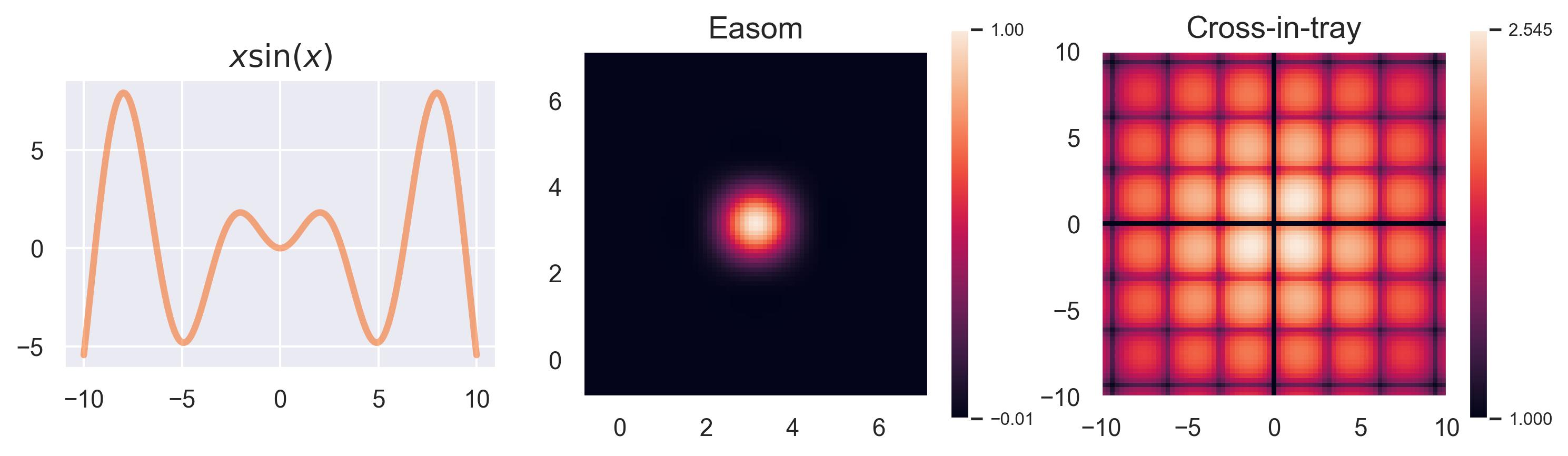
Running examples: x sin(x), Easom, and Cross-in-tray #
In this blogpost we will use three running examples to explain GPs and BO. The first one is the function
\(f(x) = x\sin(x)\)
, which is one-dimensional in its inputs and allows us to visualize how GPs handle uncertainty. The two remaining ones are part of a plethora of test functions that are usually included in black-box optimization benchmarks:1 Easom and Cross-in-tray. Their formulas are given by
We take the 2D versions of these functions for visualization, but notice how these can easily be extended to higher dimensions. The Easom test function has its optimum at
\((\pi, \pi)\)
, and the Cross-in-tray has 4 equally good optima at
\((\pm 1.35, \pm 1.35)\)
, approximately.
An introduction to Gaussian Processes #
Gaussian Processes are a probabilistic regression method. This means that they approximate a function \(f\colon\mathcal{X}\to\mathbb{R}\) while quantifying values like expectations and variances. More formally,
Definition: A function \(f\) is a Gaussian Process (denoted \(f\sim\text{GP}(\mu_0, k)\) ) if any finite collection of evaluations \(\{f(\bm{x}_1), \dots, f(\bm{x}_N)\}\) is normally distributed like
\[\begin{bmatrix} f(\bm{x}_1) \\ \vdots \\ f(\bm{x}_N) \end{bmatrix} \sim \mathcal{N}\left(\begin{bmatrix} \mu_0(\bm{x}_1) \\ \vdots \\ \mu_0(\bm{x}_N) \end{bmatrix}, \begin{bmatrix} k(\bm{x}_1, \bm{x}_1) & \cdots & k(\bm{x}_1, \bm{x}_N) \\ \vdots & \ddots & \vdots \\ k(\bm{x}_N, \bm{x}_1) & \cdots & k(\bm{x}_N, \bm{x}_N) \end{bmatrix}\right)\]The matrix \(\bm{K} = [k(\bm{x}_i, \bm{x}_j)]\) is known as the Gram matrix, and since we’re using it as a covariance matrix, this imposes some restrictions on our choice of kernel (or covariance function) \(k\) : it must be symmetric positive-definite, in the sense that the Gram matrices it spans should be symmetric positive definite. The function \(\mu_0\) is called a prior, and it allows us to inject expert knowledge in our modeling (if e.g. we know that our function should be something like a line or a parabola, we can set such \(\mu_0\) ). It’s pretty common to set \(\mu_0 \equiv 0\) (or a constant), and let the data speak for itself.
Assuming \(f\sim \text{GP}(\mu, k)\) allows for computing an entire distribution over previously unseen points. As an example, let’s say you have a dataset \(\mathcal{D} = \{(x_1, f(x_1)), \dots, (x_N, f(x_N))\}\) for our test function \(f(x)=x\sin(x)\) , measured with a little bit of noise:
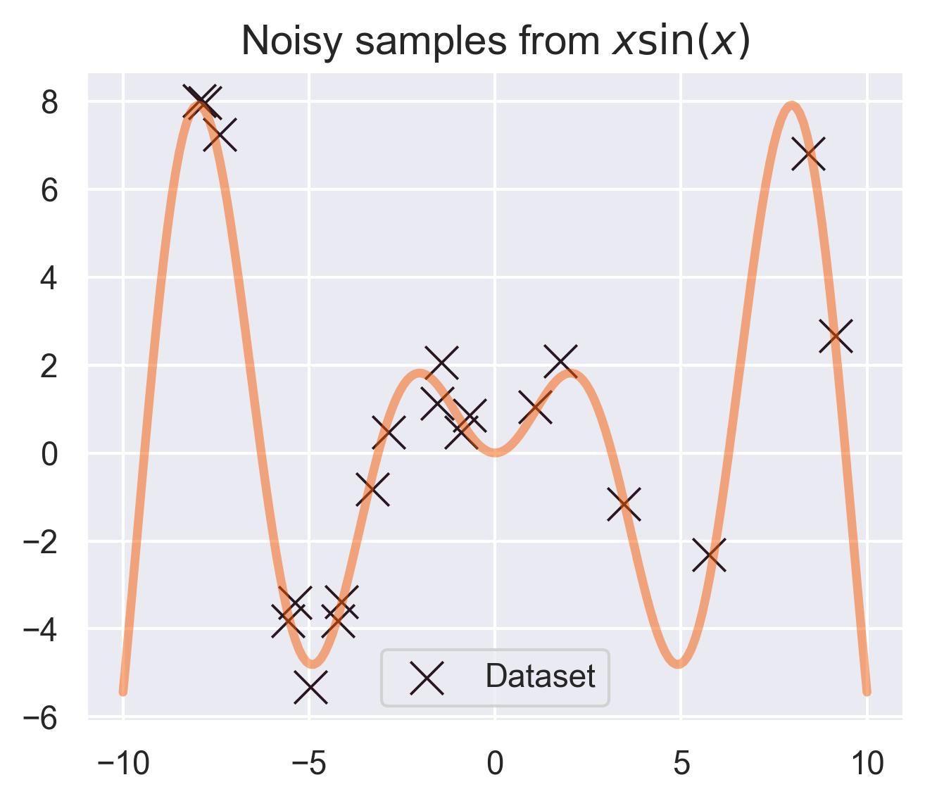
Given a new point \(x_*\) that’s not on the dataset, you can consider the joint distribution of \(\{f(x_1), \dots, f(x_N), f(x_*)\}\) and compute the conditional distribution of \(f(x_*)\) given the dataset:
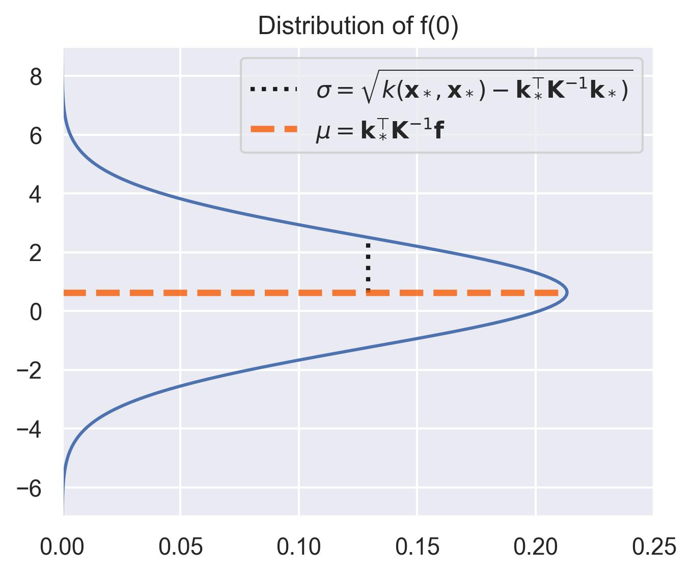
\[f(\bm{x}_*) \sim \mathcal{N}(\mu_0(\bm{x}_*) + \bm{k}_*^\top \bm{K}^{-1}(\bm{f} - \bm{\mu_0}), k(\bm{x}_*, \bm{x}_*) - \bm{k}_*^\top \bm{K}^{-1} \bm{k}_*)\]where \(\bm{k}^* = [k(\bm{x}_*, \bm{x}_i)]_{i=1}^N\) , \(\bm{f} = [f(\bm{x}_i)]_{i=1}^N\) , \(\bm{\mu_0} = [\mu_0(\bm{x}_i)]_{i=1}^N\) , and \(\bm{K}=[k(\bm{x}_i, \bm{x}_j)]_{i,j=1}^N\) .2
Consider the distribution around \(x_*=0\) in our running example, assuming that the prior \(\mu_0\) equals \(0\) . The closest values we have in the dataset are at \(x=-0.7\) and \(x=1.1\) , which means \(x_*=0\) is far away from the training set. This is automatically quantified by the variance in the posterior distribution of \(f(x_*)\) :
Let’s visualize this distribution for all points in the interval [-10, 10], sweeping through them and highlighting the actual value of the function \(f(x) = x\sin(x)\) .
Notice how the distribution spikes when close to the training points, and flattens outside the support of the data. This is exactly what we mean by uncertainty quantification.
This process of predicting Gaussian distributions generalizes to collections of previously unseen points \(\bm{X}_*\) , allowing us consider the mean prediction and the uncertainties around it. The math is essentially the same, and the details can be found in the references.
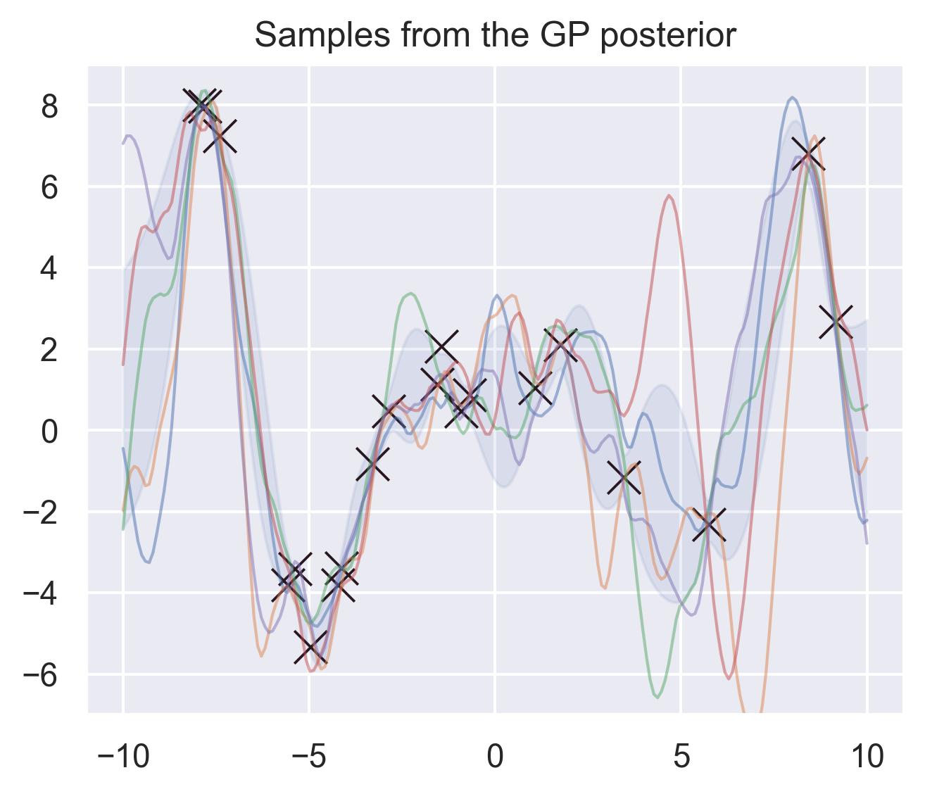
If we consider a fine enough grid of points and consider their posterior distribution, we can essentially “sample a function” out of our Gaussian Process using the same formulas described above. For example, these are 5 different samples of potential approximations of \(f(x) = x\sin(x)\) according to the posterior of the GP:
Common choices of kernels are the RBF and the Matérn family:
- \(k_{\text{RBF}}(\bm{x},\bm{x}';\; \theta_{\text{out}}, \bm{\theta}_\text{l}) = \theta_{\text{out}}\exp\left(-\frac{1}{2}r(\bm{x}, \bm{x}'; \bm{\theta}_{\text{l}})\right)\)
- \(k_\nu(\bm{x}, \bm{x}';\; \theta_{\text{out}}, \bm{\theta}_\text{l}) = \theta_{\text{out}}\frac{2^{1 - \nu}}{\Gamma(\nu)}(\sqrt{2\nu}r)^\nu K_\nu(\sqrt{2\nu}r(\bm{x}, \bm{x}'; \bm{\theta}_{\text{l}}))\)
Where
- \(r(\bm{x}, \bm{x}'; \bm{\theta}_{\text{l}}) = (\bm{x} - \bm{x}')^\top(\bm{\theta}_{\text{l}})(\bm{x} - \bm{x}')\) is the distance between \(\bm{x}\) and \(\bm{x}'\) mediated by a diagonal matrix of lengthscales \(\bm{\theta}_{\text{l}}\) , \(\theta_{\text{out}} > 0\) is a positive hyperparameter called the output scale,
- \(\Gamma\) is the Gamma function, \(K_\nu\) is the modified Bessel function of the second kind, and
- \(\nu\) is usually 5/2, but it can be any positive real number. For \(\nu = i + 1/2\) (with \(i\) a positive integer) the kernel takes a nice closed form.3
These kernels have some hyperparameters in them (like the lengthscale matrix \(\bm{\theta}_l\) or the output scale \(\theta_{\text{out}}\) ). Fitting a Gaussian Process to a given dataset consists of estimating these hyperparameters by maximizing the likelihood of the data.
To summarize,
- By using GPs, we assume that finite collections of evaluations of a function are distributed normally around a certain prior \(\mu_0\) , with covariances dictated by a kernel \(k\) .
- This assumption allows us to compute distributions over previously unseen points \(\bm{x}_*\) .
- Kernels define the space of functions we can use to approximate, and come with certain hyperparameters that we need to fit by maximizing the likelihood.
Gaussian Processes in practice #
scikit-learn #
There are several open source implementations of Gaussian Process Regression, as described above. First, there’s scikit-learn’s interface, which quickly allows for specifying a kernel. This is the code you would need to create the noisy samples described above, and to fit a Gaussian Process to those samples:
from sklearn.gaussian_process import GaussianProcessRegressor
from sklearn.gaussian_process.kernels import RBF, WhiteKernel

import numpy as np

def fit_gaussian_process(
    inputs: np.ndarray, outputs: np.ndarray
) -> GaussianProcessRegressor:
    """
    Fits a Gaussian Process with an RBF kernel
    to the given inputs and outputs.
    """

    # --------- Defining the kernel ---------
    # the "1 *" in front is understood as the
    # output scale, and will be optimized during
    # training. Besides the RBF, we also add a
    # WhiteKernel, which corresponds to adding a
    # constant to the diagonal of the covariance.
    kernel = 1 * RBF() + WhiteKernel()

    # ------ Defining the Gaussian Process -----
    # Besides the kernel, we could also specify the
    # internal optimizer, the number of iterations,
    # etc.
    model = GaussianProcessRegressor(kernel=kernel)
    model.fit(inputs, outputs)

    return model
Internally, scikit-learn uses scipy’s optimizers to maximize the likelihood w.r.t. the kernel parameters. You can check the kernel’s optimized parameters by printing model.kernel_. These are the hyperparameters for our running example on
\(f(x) = x\sin(x)\)
:
4.72**2 * RBF(length_scale=1.58) + WhiteKernel(noise_level=0.229)
And this is the predicted mean and uncertainty:
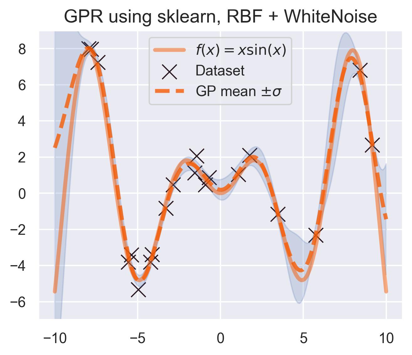
A pretty good fit! scikit-learn’s implementation is great, but it only deals with the classic exact inference, in which we solve for the inverse of the Gram matrix of all the data. This is prohibitively expensive for large datasets, since the complexity of computing this inverse scales cubically with the size of the dataset. More contemporary approaches use approximate versions of this inference.
GPyTorch #
GPyTorch was developed with other forms of Gaussian Processes in mind, plus scalable exact inference. The authors promise exact inference with millions of datapoints, and they achieve this by reducing the computational complexity of inference from \(O(n^3)\) to \(O(n^2)\) . Check their paper for more details.
Following the tutorials, this is how you would specify the same Gaussian Process we did for scikit-learn:
import torch

from gpytorch.models import ExactGP
from gpytorch.distributions import MultivariateNormal
from gpytorch.likelihoods import GaussianLikelihood
from gpytorch.means import ZeroMean
from gpytorch.kernels import ScaleKernel, RBFKernel

from gpytorch.mlls import ExactMarginalLogLikelihood


class OurGP(ExactGP):
    def __init__(
        self,
        train_inputs: torch.Tensor,
        train_targets: torch.Tensor,
        likelihood: GaussianLikelihood,
    ):
        super().__init__(train_inputs, train_targets, likelihood)

        # Defining the mean
        # The convention is to call it "mean_module",
        # but I call it mean.
        self.mean = ZeroMean()

        # Defining the kernel
        # The convention is to call it "covar_module",
        # but I usually just call it kernel.
        self.kernel = ScaleKernel(RBFKernel())

    def forward(self, inputs: torch.Tensor) -> MultivariateNormal:
        """
        The forward method is used to compute the
        predictive distribution of the GP.
        """
        mean = self.mean(inputs)
        covar = self.kernel(inputs)

        return MultivariateNormal(mean, covar)


def fit_gaussian_process(
    inputs: torch.Tensor,
    outputs: torch.Tensor,
) -> OurGP:
    """
    Fits a Gaussian Process with an RBF kernel to
    the given inputs and outputs
    """

    # ------- Defining the likelihood ----------
    # The likelihood is the distribution of the outputs
    # given the inputs and the GP.
    likelihood = GaussianLikelihood()

    # ------------ Defining the model ------------
    model = OurGP(inputs, outputs, likelihood)

    # ------------ Training the model ------------
    # The marginal log likelihood is the objective
    # function we want to maximize.
    mll = ExactMarginalLogLikelihood(likelihood, model)
    mll.train()

    # We optimize the marginal likelihood just like
    # optimize any other PyTorch model. The model
    # parameters in this case come from the kernel
    # and likelihood.
    optimizer = torch.optim.Adam(model.parameters(), lr=0.1)

    for iteration in range(3000):
        optimizer.zero_grad()
        dist_ = model(inputs)
        loss = -mll(dist_, outputs).mean()
        loss.backward()
        optimizer.step()

        if iteration % 100 == 0:
            print(f"Iteration {iteration + 1}/{3000}: Loss = {loss.item()}")

    # It is IMPORTANT to call model.eval(). This
    # will tell GPyTorch that the forward calls
    # are now inference calls, computing the
    # posterior distribution with the given
    # kernel hyperparameters.
    model.eval()

    return model
Notice that, to train a model using GPyTorch, we need to write significantly more code: specifying that the likelihood is Gaussian, defining the optimizer explicity, and optimizing the likelihood manually. This might seem verbose, but it’s actually giving us plenty of flexibility! We could e.g. include a neural network in our forward, use other likelihoods, or interplay with other PyTorch-based libraries.
You can also see the kernel hyperparameters:
print("lengthscale: ", model.kernel.base_kernel.lengthscale.item())
print("output scale: ", model.kernel.outputscale.item())
print("noise: ", model.likelihood.noise_covar.noise.item())
Which outputs something pretty similar to what scikit-learn gave us:
lengthscale:  1.5464047193527222
output scale:  20.46845245361328
white noise:  0.23084479570388794
And the predictive posterior looks like this:
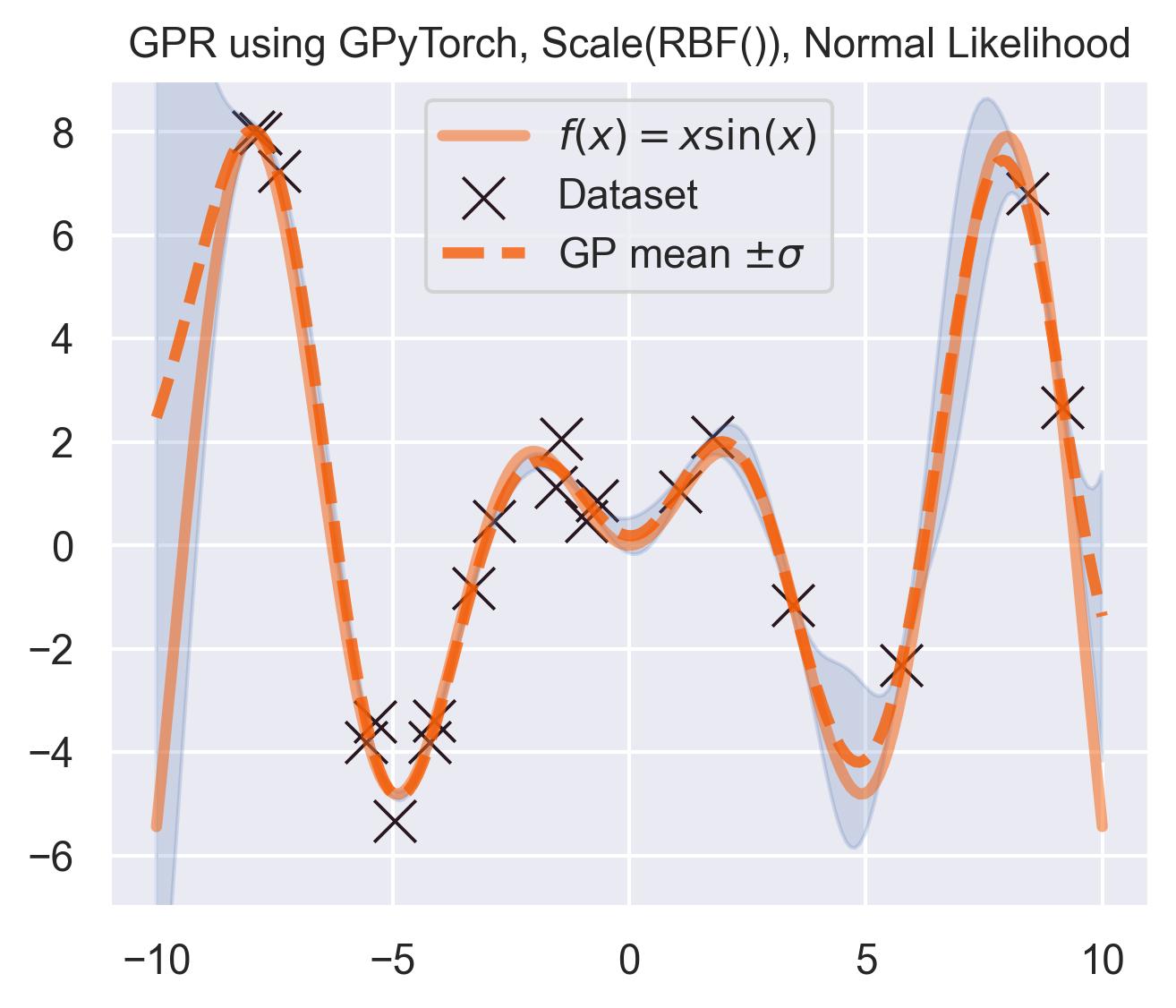
Pretty similar to scikit-learn! Which is to be expected: the equations are exactly the same, and the kernel and likelihood hyperparameters are close.
Other tools for Gaussian Process Regression #
There are three other tools for building GPs that come to mind:
- GPy, developed by Neil Lawrence and his team when he was still at Sheffield.
- GPJax, made by Thomas Pinder. Instead of using PyTorch for the backend, it uses Jax. I’d love to try it at some point!
- GPFlow, made by James Hensman and Alexander G. de G. Matthews. It uses Tensorflow as the backend.
A visual introduction to Bayesian Optimization #
Bayesian Optimization (B.O.) has three key ingredients:
- A black-box objective function \(f\colon\mathcal{X}\to\mathbb{R}\) , where \(\mathcal{X}\) is usually a subset of some \(\mathbb{R}^D\) , which we are trying to maximize. \(f\) is called the objective function.
- A probabilistic surrogate model \(\tilde{f}\colon\mathcal{X}\to\mathbb{R}\) , whose goal is to approximate the objective function. Since we will use Gaussian Processes, the ingredients we will need are a prior \(\mu_0\colon\mathcal{X}\to\mathbb{R}\) and kernel \(k\) .4
- An acquisition function \(\alpha(\bm{x}|\tilde{f})\) which measures the “potential” of new points using the surrogate model. If a given \(\bm{x}_*\in\mathcal{X}\) scores high in the acquisition function, then it potentially maximizes the objective function \(f\) .
The usual loop in a B.O. goes like this:
- Fit the surrogate model \(\tilde{f}\) to the data you have collected so far.
- Using \(\tilde{f}\) , optimize the acquisition function \(\alpha\) to find the best candidate \(\bm{x}\) (i.e. find \(\bm{x} = \arg\max \alpha(\cdot|\tilde{f})\) ).
- Query the expensive objective function on \(\bm{x}\) and repeat from 1 including this new data pair.
We usually stop after finding an optimum that is high enough, or after a fixed number of iterations.5
As we discussed in the introduction, examples of black-box objective functions include the output of expensive simulations in physics and biology, or the accuracy of an ML setup. Now we discuss four examples of acquisition functions.
Thompson Sampling #
The simplest of all acquisition functions is to sample one approximation of \(f\) and to optimize it. This can be done quite easily in most probabilistic regression methods, including Gaussian Processes.
Circling back to our guiding example of \(x\sin(x)\) , let’s start by only having \(\mathcal{D}_{\text{init}} = \{(0, f(0))\}\) in our dataset, and iteratively query the next proposal suggested by Thompson sampling:
At first, the samples are not approximating the objective function at all, and so we end up exploring the domain almost at random. These initial explorations allow us to get a better approximation of the function. TS quickly finds the left optimum, and tends to get stuck there, since further samples are likely to have their maximum there.
Improvement-based policies #
Since we have estimates of the posterior mean \(\mu\) and the posterior variance \(\sigma^2\) at each step, we have access to a lot more than just a single sample (as in TS): we can query for probabilistic quantities such as expectations or probabilities.
For each new point \(\bm{x}_*\) , consider its “improvement”:
\[ I(\bm{x}_*; \mathcal{D}) = \max(0, f(\bm{x}_*) - f_{\text{best}})\]where \(f_{\text{best}}\) is the maximum value for \(f(\bm{x}_n)\) in our trace \(\mathcal{D} = \{(\bm{x}_n, f(\bm{x}_n))\}_{n=1}^N\) . The improvement measures how much we are gaining at point \(f(\bm{x}_*)\) , compared to the current best.
since we have a probabilistic approximation of \(f\) , we can compute quantities like the probability of improvement (PI):
\[\alpha_{\text{PI}}(\bm{x}_*; \mathcal{D}) = \text{Prob}[I(\bm{x}_*;\mathcal{D}) > 0] = \text{Prob}[f(\bm{x}_*) > f_{\text{best}}],\]In other words, PI measures the probability that a given point will be better than the current maximum. Another quantity we can measure is the expected improvement (EI)
\[ \alpha_{\text{EI}}(\bm{x}_*; \mathcal{D}) = \mathbb{E}[I(\bm{x}_*;\mathcal{D})]\]which measures by how much a given \(\bm{x}_*\) may improve on the current best.6
Using the same running example and sample we showed for TS, here’s how EI fairs:
Notice that the right size of this plot now shows the values for \(\alpha_{\text{EI}}\) in a different scale. At first, all points have almost the same expected improvement (since we haven’t explored the function at all, and so we are uncertain). Querying the maximum of \(\alpha_{\text{EI}}\) iteratively allows us to find not only the left optimum, but also the right one!
Upper-Confidence Bound #
Another type of acquisition function is the Upper-Confidence Bound (UCB), which optimistically chooses the points are on the upper bounds of the uncertainty. More explicitly, let \(\mu\) and \(\sigma\) be the posterior mean and standard deviation on a given point \(\bm{x}\) after fitting the GP, then
\[ \alpha_{\text{UCB}}(\bm{x}_*; \mathcal{D}, \beta) = \mu(\bm{x}_*) + \beta\sigma(\bm{x}_*), \]where \(\beta > 0\) is a hyperparameter that states how optimistic we are on the upper bound of the variance. High values of \(\beta\) encourage exploration (i.e. exploring regions with higher uncertainty), while lower values of \(\beta\) encourage exploitation (staying close to what the posterior mean has learned). To showcase the impact of this hyperparameter, here are two versions of BO on our running example: one with \(\beta=1\) , and another with \(\beta=5\) .
Notice that, for \(\beta=1\) , the optimization gets stuck on the first global optima. This doesn’t happen for \(\beta=5\) :
Bayesian Optimization in practice: BoTorch #
BoTorch is a Python library that interoperates well with GPyTorch for running BO experiments. All the animations I presented above were made by fitting BoTorch’s models for exact GP inference, and by using their implementations of the acquisition functions (except for Thompson Sampling).
Following their tutorial (and adapting it to our example), this is a minimal working version of the code for doing a Bayesian Optimization loop:
from typing import Callable, Tuple

import torch
from gpytorch.mlls import ExactMarginalLogLikelihood
from gpytorch.means import ZeroMean

# Single Task GP is a Gaussian Process on one value,
# using certain defaults for kernel and mean.
# mean: a constant that gets optimized.
# kernel: Matérn 5/2 kernel with output scale.
from botorch.models import SingleTaskGP

# BoTorch provides tools for fitting these
# models easily.
from botorch.fit import fit_gpytorch_model

# Using the UCB acquisition function
from botorch.acquisition import UpperConfidenceBound


def bayesian_optimization(
    objective_f: Callable[[float], float],
    n_iterations: int = 20,
) -> Tuple[torch.Tensor, torch.Tensor]:
    # Some hyperparameters
    ACQ_BETA = 1.0
    domain = torch.linspace(-10, 10, 200)

    # Querying at 0
    # This could be modified to sample at random
    # from the domain instead.
    inputs_trace = [torch.Tensor([0])]
    outputs_trace = [objective_f(inputs_trace[-1])]

    for _ in range(n_iterations):
        # Consolidating the inputs and outputs
        # for this iteration
        inputs = torch.Tensor(torch.cat(inputs_trace))
        outputs = torch.Tensor(torch.cat(outputs_trace))

        # --- Fitting the GP using BoTorch's tools ---
        # Defining the model.
        # Instead of using the constant mean given by
        # BoTorch as a default, we go for a zero mean.
        gp_model = SingleTaskGP(
            inputs.unsqueeze(1),
            outputs.unsqueeze(1),
            mean_module=ZeroMean(),
        )

        # Defining the marginal log-likelihood
        mll = ExactMarginalLogLikelihood(
            gp_model.likelihood,
            gp_model,
        )

        # Maximizing the log-likelihood
        fit_gpytorch_model(mll)

        gp_model.eval()

        # ---- Maximizing the acquisition function -----
        acq_function = UpperConfidenceBound(model=gp_model, beta=ACQ_BETA)
        # BoTorch expects the input to be
        # of shape (b, 1, 1) in this case.
        acq_values = acq_function(domain.reshape(-1, 1, 1))

        # The next candidate is wherever the
        # acquisition function is maximized
        next_candidate = domain[acq_values.argmax()]

        # ---- Querying the obj. function ---------
        inputs_trace.append(
            torch.Tensor([next_candidate])
        )
        outputs_trace.append(
            torch.Tensor([objective_f(next_candidate)])
        )

    return (
        torch.Tensor(torch.cat(inputs_trace)),
        torch.Tensor(torch.cat(outputs_trace)),
    )
Bayesian Optimization loops for Easom and Cross-in-Tray #
Bayesian Optimization works for black-box objective function with general domains
\(\mathcal{X}\subseteq\mathbb{R}^D\)
. To showcase this, we can run BO in
\(\mathbb{R}^2\)
on the test functions Easom and Cross-in-tray:
Cross-in-tray is a particularly difficult function for black-box optimization algorithms based on Evolutionary Strategies.7 Let me show you e.g. CMA-ES trying to optimize it:
Unless it gets lucky with the initialization, CMA-ES tends to get stuck in one of the many local optima of Cross-in-tray. Of course, there are ways to encourage more exploration in Evolutionary Strategies, but this is something that is accounted for automatically in BO.
Another advantage of BO vs. Evolutionary Strategies is sample efficiency: for each generation, an evolutionary strategy must query the objective function as many times as the population size. This is prohibitively expensive if the objective function is e.g. an expensive simulation that cannot be run in parallel.8
Bayesian Optimization’s drawbacks #
Bayesian Optimization is a major achievement of Bayesian statistics. It, however, has major drawbacks and hidden assumptions. Let’s list a couple of them:
How do we optimize the acquisition function? #
You might have noticed that, in our running example, we optimized the acquisition function by evaluating it on the entire domain, and then querying its maximum (i.e. we just did a grid search). This obviously doesn’t scale to higher dimensions!
There are several alternatives to this. Since we can evaluate the acq. function easily, we could simply use Evolutionary Strategies (like CMA-ES, shown above) to optimize it. Otherwise, we could rely on gradient-based optimization.9
Other alternatives to high dimensional inputs focus on running the optimization of the acquisition function on only trust regions, centered around the best performing points. These trust regions are essentially small cubes, whose size adapts over the optimization.
(Exact) Gaussian Processes don’t scale well #
Vanilla versions of kernel methods and Gaussian Processes don’t scale well with either the size of the dataset, or the dimension of the input space. Folk knowledge says that (vanilla) Gaussian Processes don’t fit well above 20 input dimensions.10
When it comes to large datasets, exact GP inference may be possible with GPyTorch and their implementation. Approximate inference is usually done through inducing points, which are a set of points that’s representative of the entire dataset.11
High dimensional inputs are usually projected to lower-dimensional spaces, using either linear mappings (assuming e.g. that there are several dimensions that are uninformative and can be ignored), or using neural networks. Another alternative is to provide a handcrafted mapping from solution to a so-called behavior space (as they do in the Intelligent Trial-and-Error paper, using MAP-Elites).12
Parallelizing #
As formulated above, BO is sequential in nature: we fit a surrogate model to the current dataset, we use this surrogate model to construct an acquisition function, which we optimize to get the next point. Parallelizing BO isn’t trivial, and the literature shows that the principled ways for parallelization are highly dependant on the acquisition function. See the references for more details.
Stopping criteria #
A problem that is transversal to black-box optimization algorithms is knowing when to stop. Most practitioners just have a fixed amount of compute, or decide to stop when they have found a solution that is “good enough” for them (e.g. a hyperparameter search that’s above a certain accuracy).
There are theory-driven ways to solve this problem. Gaussian Processes allows for computing notions of “regret”, which are being used to define optimization processes that stop automatically.
Conclusion #
Bayesian Optimization lets you optimize black-box functions (i.e. functions that have no closed form, and are expensive to query) by approximating them using a probabilistic surrogate model. In this blogpost, we explored using Gaussian Processes as surrogates, and several acquisition functions that leverage the uncertainties that GPs give. We briefly showed how these different acquisition functions explore and exploit the domain to find a suitable optimum.
When compared to e.g. Evolutionary Strategies, we briefly saw how CMA-ES might get stuck in local optima if the landscape is tough. BO is also more sample efficient, since Evolutionary Strategies need to query the objective function in entire populations at each generation.
We wrapped up by discussing some of the drawbacks of BO: optimizing the acquisition function is not trivial in high dimensions, Gaussian Processes rely on approximations to fit large or high dimensional datasets, and parallelization depends highly on the choice of acquisition function.
Cite this blogpost #
If you found this blogpost useful, feel free to cite it.
@online{introToBO:Gonzalez-Duque:2023,
  title = {Bayesian Optimization using Gaussian Processes: an introduction},
  author = {Miguel González-Duque},
  year = {2023},
  url = {https://miguelgondu.com/blogposts/2023-04-08/intro-to-bo}
}
References #
Gaussian Processes #
- Gaussian Processes for Machine Learning by Rasmussen and Williams. Chapters 2, 4 and 9. This book is “the bible” of Gaussian Processes.
- Probabilistic Numerics by Hennig, Osborne and Kersting. Secs. 4.2 and 5.5. I really like their presentation of Gaussian algebra and of Gaussian Processes. The computations for the posterior GP can be found either here or in the bible.
- A Unifying View of Sparse Approximate Gaussian Process Regression, by Quiñonero-Candela and Rasmussen. A paper about inducing points/active sets/pseudo-inputs in GPs.
- Exact Gaussian Processes on a Million Data Points.
Bayesian Optimization #
- Taking the human out of the loop: a review of Bayesian Optimization, by Shahriari et al.. What a classic.
- Maximizing acquisition functions for Bayesian optimization, by Wilson, Hutter and Deisenroth. This paper discusses how to approximate the gradients of acquisition functions using MC, and leveraging differentiable kernels.
- Scalable Global Optimization via Local Bayesian Optimization, by Eriksson et al.. This paper introduces
TurBO, or Bayesian Optimization with trust regions. - Maximilian Balandat has several papers on parallel versions of Bayesian Optimization. Check his google scholar for some examples.
- The stopping criteria is currently under plenty of research. Check for example the work of Anastasiia Makarova. In particular Automatic Termination for Hyperparameter Optimization.
- Robots that can adapt like animals, by Cully et al. A great example of Bayesian Optimization on top of handcrafted features.
-
(Optimization benchmarks) There are plenty more test functions for optimization in this link. ↩︎
-
(the ugly details) I will skip the ugly details in this blogpost. The computation of a Gaussian Process’ predictive posterior can be found in Sec. 2.2. of Gaussian Processes for Machine Learning, by Rasmussen and Williams, or on Sec. 4.2.2. of Probabilistic Numerics, by Hennig et al.. Notice that I’m skipping the discussion on diagonal noise modeling. ↩︎
-
(details on Matérn) For more details, see Probabilistic Numerics, Sec. 5.5.. ↩︎
-
(other surrogate models) We are using Gaussian Processes as a surrogate model here, but other ones could be used! The main requirement is for them to allow us to have good uncertainty estimates of the objective function. Recent research by Yucen Lily Li, Tim Rudner and Andrew Gordon Wilson has explored this direction. ↩︎
-
(stopping criteria) It’s not so simple. The stopping criteria of BO are a topic that is currently under plenty of research. See the references. ↩︎
-
(closed form) These two acquisition functions have closed form when we use vanilla Gaussian Processes. For the technical details, check the references. ↩︎
-
(David Ha’s blogpost) If you’re not familiar with evolutionary strategies, I can’t recommend David Ha’s introduction enough. ↩︎
-
(sample efficiency comparison) In Sec. 3.4. of my dissertation I run a sample-efficiency comparison between BO and CMA-ES for these two test functions. The results show that BO reliably finds an optima in less queries to the objective function. I plan to run experiments on higher-dimensional examples in the future. ↩︎
-
(GPs are differentiable) Depending on our choice of kernel, we can also compute distributions over the gradient of a Gaussian Process. I would love to dive deeper here, but I think it’s a topic on its own. Check Sec. 9.4. of Gaussian Processes for Machine Learning or this paper on estimating gradients of acquisition functions for more details. ↩︎
-
(folk) Check for example this Stack Exchange question. ↩︎
-
(inducing points) The classic reference to cite for inducing points is a paper by Quiñonero-Candela and Rasmussen. Check it if you’re interested! ↩︎
-
(intelligent trial-and-error) See Robots that can adapt like animals, by Cully et al. The authors learn a corpus of different robot controllers using handcrafted dimensions, and then adapt to damage using Bayesian Optimization. ↩︎