Mapping high-dimensional Bayesian optimization using small molecules
June 21, 2024
It is written that animals are divided into
- those that belong to the Emperor,
- embalmed ones,
- those that are trained,
- suckling pigs,
- mermaids,
- fabulous ones,
- stray dogs,
- those that are included in this classification,
- those that tremble as if they were mad,
- innumerable ones,
- those drawn with a very fine camel’s hair brush,
- others,
- those that have just broken a flower vase,
- those that resemble flies from a distance.
[…] I have noted the arbitrariness of Wilkins, of the unknown (or apocryphal) Chinese encyclopedist, and of the Bibliographical Institute of Brussels; obviously there is no classification of the universe that is not arbitrary and conjectural.
The Analytical Language of John Wilkins, by Jorge Luis Borges. Other Inquisitions 1937-1952. Translated by Ruth L.C. Simms.
Introduction #
Bayesian optimization (BO) shows great promise for several tasks: It is used for automating the development of Machine Learning models, building self-driving labs, and creating new materials.1
These tasks often involve high-dimensional inputs with a lot of structure. Two examples: to derive a chemical compound you need to modulate several variables at the same time: the pH and type of the solvent, the amount of different solutions to mix in, the temperature, the pressure… or to quickly optimize a Machine Learning model to the best accuracy possible, you might need to modulate the choice of opimizer, the learning rate, the number and types of layers and neurons.
We need, then, high-dimensional Bayesian optimization over highly structured inputs. High-dimensional BO (HDBO) is a large research field, and we recently wrote a paper with an updated survey and taxonomy composed of 7 families of methods:
- Variable Selection: choosing only a subset of variables and optimizing there.
- Linear embeddings: Optimizing in a linear subspace,
- Trust regions: Limiting the optimization of the acquisition function to a small cube in the high-dimensional space,
- Gradient information: Using information from the gradient predicted by the underlying GP,
- Additive models: Decomposing the objective function into a sum of functions with less variables,
- Non-linear embeddings: Using e.g. neural networks to learn latent spaces and optimizing therein,
- Structured Spaces: working directly with the structured representations (e.g. using tools from differential geometry, or discrete optimization).
Here’s a visual overview (click it for a version with links to all the references and open source implementations):
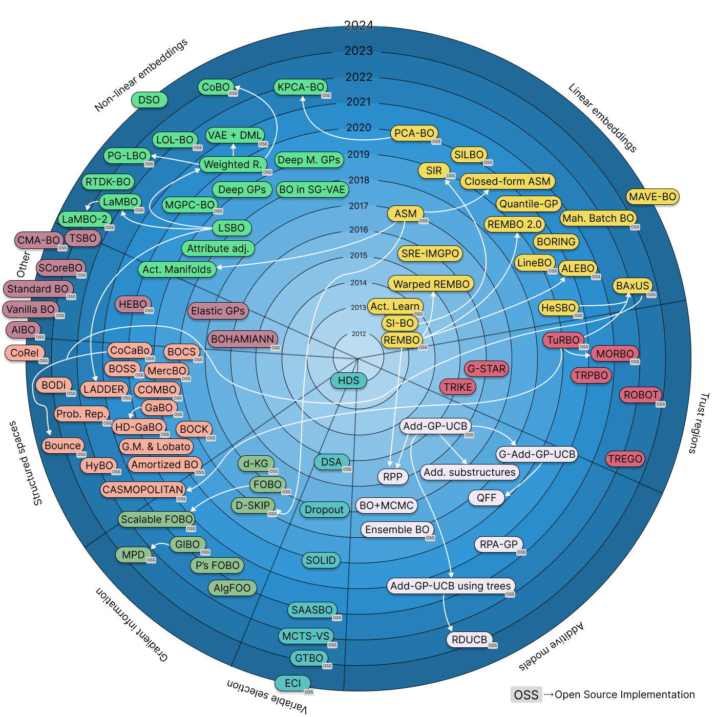
A timeline and taxonomy of high-dimensional Bayesian optimization. Click it for an interactive version with links to papers and open source implementations.
In this blogpost and the ones that follow I will dive into this taxonomy and each of the families. The final goal is to provide a map of HDBO: a comprehensive overview, tutorialized with code. This blogpost in particular presents an introduction to HDBO, and a couple of baselines. The next ones will dive into the families of the taxonomy.
I want to emphasize that I’m building on prior work done by Binois & Wycoff, as well as Santoni et al.’s comparison of HDBO methods. The taxonomy shown here is an extention of what’s proposed in these two papers.
Our focus: discrete sequence optimization #
I plan to focus this overview on discrete sequence optimization problems. In these, we explore a space of “words” of length \(L\) . Of the problems mentioned above, drug discovery and protein engineering can be framed as discrete sequence optimization problems: both small molecules and proteins can be represented as sentences, as we will see later in this post.
Let’s formalize what we mean: consider a vocabulary of tokens \(v_1, \dots v_V\) . We are trying to optimize a function \(f\colon\mathcal{X}_L\to\mathbb{R}\) where \(\mathcal{X}_L = \{\bm{s} = (s_1,\dots, s_L) | s_i \in \{v_1,\dots, v_V\}\}\) is the space of sentences of length \(L\) . Our goal is finding \[\argmax_{\bm{s}\in\mathcal{X}_L} f(\bm{s}),\] i.e. finding the best performing sentence.
The next section introduces a guiding example we will use for this blogpost and the ones that follow.
A guiding example: small organic molecules #
One example of a discrete sequence optimization problem that is highly relevant for drug discovery is small molecule optimization. We could, for example, optimize small molecules such that they bind well to a certain receptor, or active site in a protein.
We can represent molecules in several ways (e.g. as graphs, as 3D objects…).2 Here, we focus on the SELFIES representation: SELFIES represent organic molecules using tokens like [C] or [N] or [Br] to represent atoms, [Branch1] to represent branching structures, and more. Aspuru-Guzik and the original authors have a great blogpost explaining how SELFIES is actually a formal grammar, made in such a way that all possible combinations of SELFIES tokens are valid molecules (a fact that doesn’t hold for SELFIES predecessor: SMILES).3
You can find the SMILES representations of e.g. aspirine by checking on PubChem:
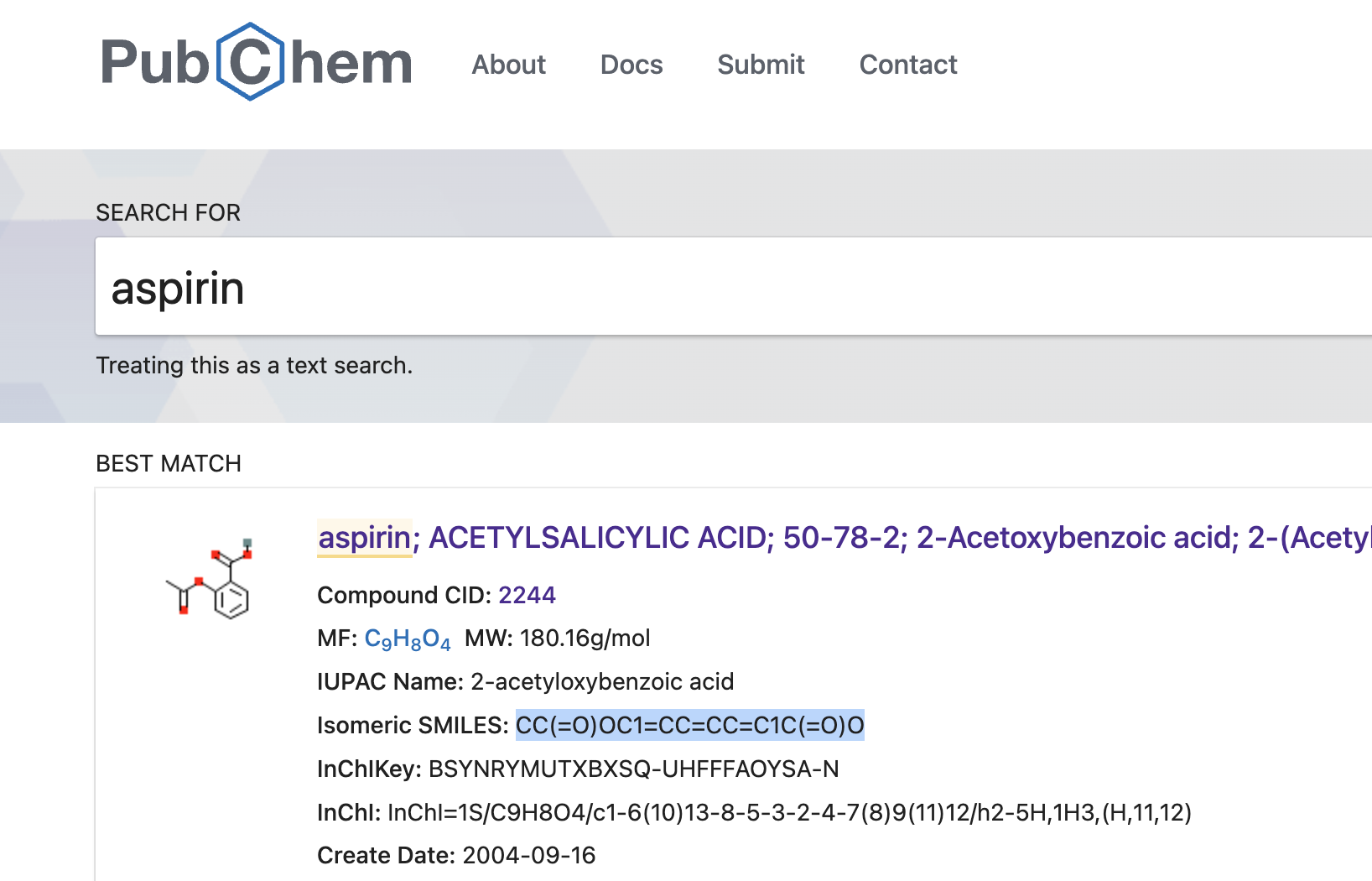
According to PubChem, aspirin's SMILES is CC(=O)OC1=CC=CC=C1C(=O)O.
And you can transform between SMILES and SELFIES using the Python package selfies, developed by Aspuru-Guzik’s lab. It is completely trivial to transform SMILES to SELFIES using it:
import selfies as sf

# Transforming aspirin's SMILES to SELFIES
aspirin_as_selfies = sf.encoder("CC(=O)OC1=CC=CC=C1C(=O)O")
print(aspirin_as_selfies)
Aspirin’s SELFIES representation is given by [C][C][=Branch1][C][=O][O][C][=C][C][=C][C][=C][Ring1][=Branch1][C][=Branch1][C][=O][O].
In these blogposts, we will work on the Zinc250k dataset. Zinc is a database of around 720k commercially available molecules, and it was originally provided by Irwin and Shoichet in 2006. Zinc250k is a subset of around 250k molecules, and it is used plenty when benchmarking generative modeling of molecules.
Zinc250k can easily be downloaded using TorchDrug in several of the representations mentioned above. We transform these SMILES into SELFIES, store the maximum sequence length, and the keep the entire alphabet used (which turned out to be made of 64 tokens).4
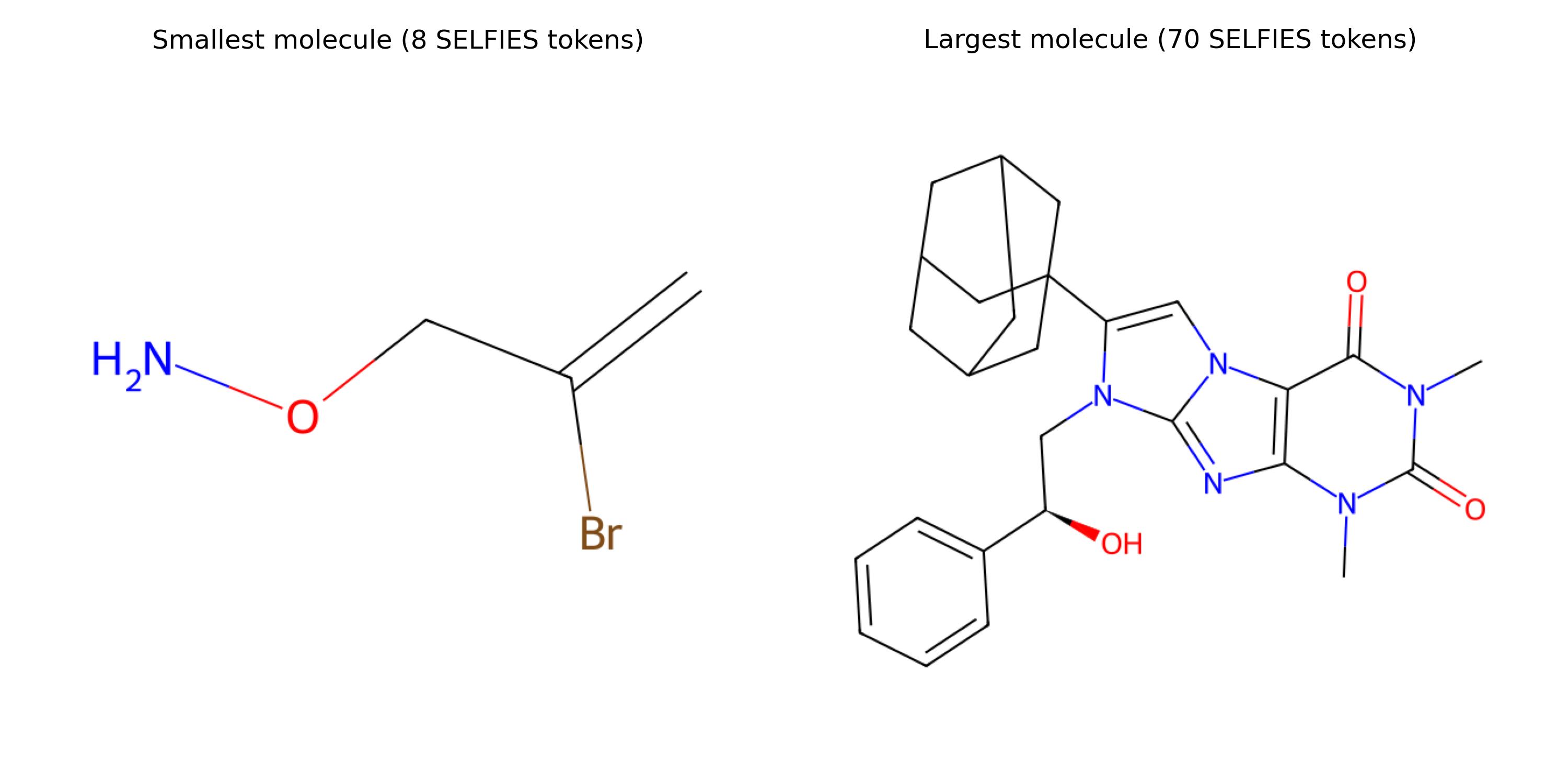
Smallest and largest molecules in terms of their SELFIES tokens.
Here are the smallest and largest molecules w.r.t. their number of SELFIES tokens. The smallest one is [C][=C][Branch1][C][Br][C][O][N], and the largest one has 70 tokens.5 We will pad all sequences in this dataset until this maximum length using the padding token [nop].
In the formal maths that we introduced in the previous section, \(v_1, \dots v_V\) correspond to the \(V=64\) unique tokens, and \(\mathcal{X}_L\) corresponds to all the sequences with length \(L=70\) .
The search space \(\mathcal{X}_L\) is enormous. Enumerating it would take all the humans that have ever existed way longer than the age of the universe. Looking at the combinatorics of it, we have 70 possible locations, and for each we have 64 possible values: \(70^{64}\) possible SELFIES sentences.6
Optimizing small molecules (or the PMO benchmark) #
We have defined our search space \(\mathcal{X}_L\) , now we’re missing examples of objective functions \(f\colon\mathcal{X}_L\to\mathbb{R}\) .
Molecular optimization is a hot topic. Several collections of black box functions have been developed in these last years. At first, we used to optimize relatively simple metrics like the Quantitative Estimate of Druglikeness (QED) or log-solubility (LogP) (see e.g. Gómez-Bombarelli et al, 2018). Attention quickly turned into more complex objectives, with Brown et al. proposing GuacaMol: a benchmark of several black box functions for molecule optimization. Soon after, Gao et al. extended this benchmark by proposing Practical Molecular Optimization (PMO), focusing on sample efficiency.7
GuacaMol and PMO include several different families of black-box objectives (e.g. being similar to a certain well-known medicine, or matching a given molecular formula). It’s worth noting that these black-boxes often rely on simple calculations over the molecule, or on data-driven oracles. They are often instant to query, which is not ideal for our setting: we might grow lazy and get the wrong impression of the speed of our algorithms, especially when actual applications can be in the timeframe of weeks or months per evaluation of the black box.
We will optimize small molecules on the PMO benchmark throughout these blogposts. Hopefully we’ll also turn our attention to other problems, like optimizing mutations of a protein wildtype.
The “worst” baseline: sampling at random #
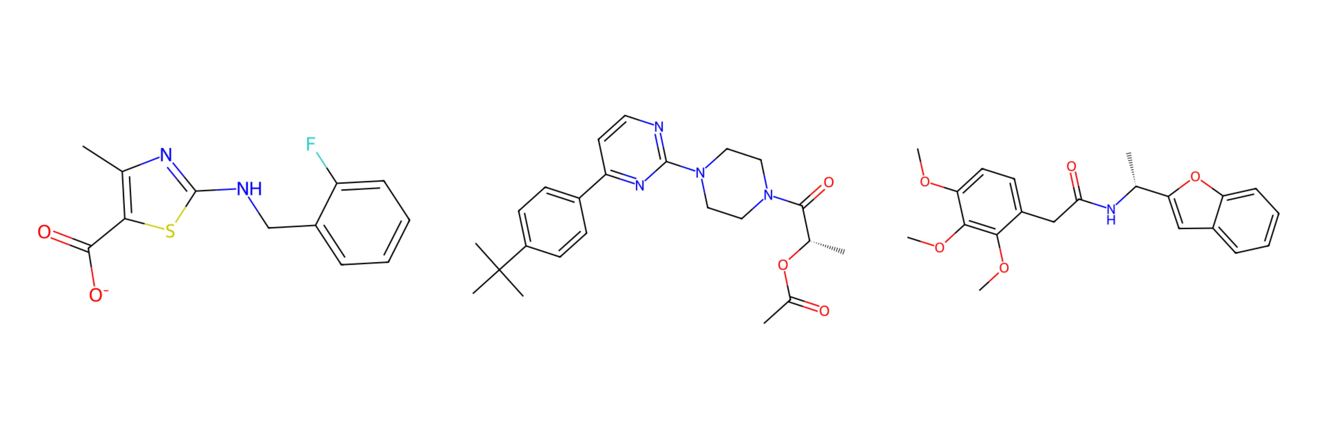
One of the silliest ways to optimize a black-box objective \(f\colon\mathcal{X}_L\to\mathbb{R}\) is to consider randomly sampled sentences. Let me show you some examples of what happens when we sample random SELFIES from our alphabet:
Three molecules made by concatenating 70 random SELFIES tokens together. Of course: they don't make any sense.
We can implement such a solver easily. Here we will use a framework for benchmarking black boxes I’ve been developing called poli-baselines:8
import numpy as np
from poli_baselines.core.abstract_solver import AbstractBlackBox, AbstractSolver

from utils import load_alphabet


class RandomSampler(AbstractSolver):
    def __init__(
        self,
        black_box: AbstractBlackBox,
        alphabet: list[str],
        max_sequence_length: int,
        x0: np.ndarray | None = None,
        y0: np.ndarray | None = None,
    ):
        super().__init__(black_box, x0, y0)
        self.alphabet = alphabet
        self.max_sequence_length = max_sequence_length
        self.history = {"x": [], "y": []}

    def _random_sequence(self) -> np.ndarray:
        # Samples a seq. of length self.max_sequence_length
        # from the alphabet self.alphabet at random.
        random_tokens = np.random.choice(self.alphabet, self.max_sequence_length)
        return np.array(["".join(random_tokens)])

    def solve(
        self,
        max_iter: int = 100,
        n_initial_points: int = 0,
        seed: int | None = None,
    ) -> None:
        if seed is not None:
            np.random.seed(seed)

        for _ in range(max_iter):
            sequence = self._random_sequence()
            val = self.black_box(sequence)

            self.history["x"].append(sequence)
            self.history["y"].append(val)

            print(f"Sequence: {sequence}, Value: {val}")
Let’s try to optimize one of the black-boxes inside PMO: finding a molecule that is similar to Albuterol, using PyTDC and poli.
To keep testing homogeneous, let’s give every algorithm we will test in these blogposts the same evaluation budget, as well as the same initialization and max. runtime.
from poli.repository import AlbuterolSimilarityBlackBox

black_box = AlbuterolSimilarityBlackBox(string_representation="SELFIES")
alphabet = load_alphabet()
max_sequence_length = 70
seed = 42

random_sampler = RandomSampler(black_box, alphabet, max_sequence_length)

random_sampler.solve(max_iter=10 + 500, seed=seed)

# Printing the best performing molecule
best_value_idx = np.argmax(random_sampler.history["y"])
best_sequence = random_sampler.history["x"][best_value_idx]
best_value = random_sampler.history["y"][best_value_idx]

print(f"Best sequence: {best_sequence}")
print(f"Best value: {best_value}")
Here’s the result of just randomly sampling sentences of SELFIES tokens for 500 iterations (with an “initialization” of 10 evaluations).
The performance of randomly sampling in albuterol_similarity.
As far as baselines go, this one is the most naïve. It is surprisingly powerful at times, and given enough budget it can surpass whatever other technique. Here, the performance can get pretty high because there’s plenty of heavy lifting being done by the SELFIES encoding. If we were to optimize on SMILES space, I would assume several of our samples would correspond to gibberish.
A less silly baseline: discrete hill-climbing #
Instead of randomly sampling each time, why don’t we just take the best performing model and mutate it at random? Let’s implement this simple logic in poli-baselines again:
class DiscreteHillClimbing(AbstractSolver):
    def __init__(
        self,
        black_box: AbstractBlackBox,
        alphabet: list[str],
        max_sequence_length: int,
        x0: np.ndarray | None = None,
        y0: np.ndarray | None = None,
    ):
        super().__init__(black_box, x0, y0)
        self.alphabet = alphabet
        self.max_sequence_length = max_sequence_length

        self.history = {
            "x": [x_i.reshape(1, -1) for x_i in x0] if x0 is not None else [],
            "y": [y_i.reshape(1, -1) for y_i in y0] if y0 is not None else [],
            "best_y": (
                [np.max(y0[: i + 1]).reshape(1, -1) for i in range(len(y0))]
                if y0 is not None
                else []
            ),
        }

    def solve(
        self,
        max_iter: int = 100,
        n_initial_points: int = 0,
        seed: int | None = None,
    ) -> None:
        if seed is not None:
            np.random.seed(seed)

        for _ in range(max_iter):
            best_idx_so_far = np.argmax(self.history["y"])
            best_sequence_so_far = self.history["x"][best_idx_so_far].reshape(1, -1)

            # Randomly select a position to mutate
            position_to_mutate = np.random.randint(self.max_sequence_length)

            # Randomly select a new token
            new_token = np.random.choice(self.alphabet)

            # Mutate the best sequence so far
            new_sequence = best_sequence_so_far.copy()
            new_sequence[0, position_to_mutate] = new_token

            # Evaluate the new sequence
            val = self.black_box(new_sequence)

            # Update the history
            self.history["x"].append(new_sequence)
            self.history["y"].append(val)
            self.history["best_y"].append(max(val, self.history["best_y"][-1]))

            print(f"Sequence: {new_sequence}, Value: {val}")
It performs slightly better than just randomly sampling.
Comparing randomly sampling with discrete hill-climbing.
And I do expect to see a lot of variance if we were to change the seed each time.
This is actually a very rudimentary version of a genetic algorithm in which we’re only selecting the best element for mutation. If we were thorough, we would actually implement a proper genetic algorithm here. It’s worth noting that mol-ga (a relatively simple genetic algorithm designed for SMILES) is allegedly performing better than all the 25 methods originally tested in the PMO benchmark. Check the paper by Tripp and Hernández-Lobato here.
Can we optimize SELFIES using Bayesian Optimization? #
A first attempt at optimizing in \(\mathcal{X}_L\) using Bayesian optimization would be to transform this discrete problem into a continuous one. We will dive deeper on how to do this in the non-linear embeddings and structured spaces families, but for now let’s do the simplest alternative: running Bayesian optimization in one-hot space.
By one-hot space, we mean encoding a given sequence as a collection of vectors \(\bm{s} = (s_1, \dots, s_L) \mapsto \bm{X} = (\bm{x}_1, \dots, \bm{x}_L)\) where each \(\bm{x}_i\) is a vector of length \(V\) with 1 at the index of the corresponding token \(s_i\) and 0 otherwise.
Notice that \(\bm{X}\) is pretty large: if we flatten it, it will be a vector of length \(L * V = 70 * 64 = 4480\) . Remember that GPs start struggling at around 30 dimensions (depending on the training set-up and the amount of data). As we discussed in the previous blogpost about vanilla Gaussian Processes, we will need plenty of samples to even fit such a surrogate model.9
Still, let’s build a simple Bayesian Optimization loop in this space, and see how it fairs. In particular, I will use a state-of-the-art high-dimensional Bayesian optimization method: Hvarfner’s Vanilla BO. I’ll leave the implementation out of the main text (you can find it in the code companion, and I’m happy to discuss them in detail if you’re interested). Here’re the results in comparison:
Comparing Hvarfner's vanilla BO against the two other baselines.
In this specific example, Hvarfner’s Vanilla BO performs roughly as well as random sampling. It’s worth highlighting that we’re only doing one repetition. I expect the other baselines to have high variance in their performance. We also note that the other baselines ran almost instantly, while these 500 iterations of BO took a little bit over an hour on my M2 Mac.
What comes next? Aternatives for high-dimensional BO #
It’s understandable that standard Bayesian optimization is not performant in the one-hot space of our set-up. A 4480-dimensional continuous search space is awfully large for GPs. In the coming blogposts we’ll dive into the families of the taxonomy we recently proposed, and measure how they fair against these simple baselines.
Here’s the plan: I will start by discussing methods that explore structured spaces. Most of these work directly on the discrete representations. Afterwards, I will dive into non-linear embeddings and on how using latent representations makes the optimization easier. These continuous latent spaces will open the doors for all the other families as well.
Conclusion #
In this blogpost I briefly introduced a taxonomy of high-dimensional Bayesian optimization methods, building on the work of Santoni et al. and Binois & Wycoff. The goal for the next blogposts is to dive deeper into the different families, building a map of high-dimensional Bayesian optimization.
Small molecules can be represented as discrete sequences (be it as SELFIES or as SMILES strings), and we will use them as a guiding example while we build this map.
This blogpost also introduces two simple baselines, and compares standard BO on one-hot representations of discrete sequences. Results show that standard BO is not as competitive, which is understandable given the size and nature of the continuous space that is being explored.
Next blogposts will explore HDBO methods that leverage structured spaces and non-linear embeddings.
-
If you need a refresher on Bayesian optimization, check the blogpost I wrote a couple of months ago. ↩︎
-
Here is a survey on small molecule representations and generative modeling in case you’re curious. Sec. 2 discusses several different ways to represent small molecules. ↩︎
-
Let me also show you the entire vocabulary for SELFIES we use, which is computed from the Zinc250k dataset:
'[nop]', '[C]', '[=C]', '[Ring1]', '[Branch1]', '[N]', '[=Branch1]', '[=O]', '[O]', '[Branch2]', '[Ring2]', '[=N]', '[S]', '[#Branch1]', '[C@@H1]', '[C@H1]', '[=Branch2]', '[F]', '[#Branch2]', '[Cl]', '[#C]', '[NH1+1]', '[P]', '[O-1]', '[NH2+1]', '[Br]', '[N+1]', '[#N]', '[C@]', '[NH3+1]', '[C@@]', '[=S]', '[=NH1+1]', '[N-1]', '[=N+1]', '[S@]', '[S@@]', '[I]', '[S-1]', '[=NH2+1]', '[=S@@]', '[=S@]', '[=N-1]', '[P@@]', '[P@]', '[NH1-1]', '[=O+1]', '[=P]', '[=P@@]', '[=OH1+1]', '[=P@]', '[#N+1]', '[S+1]', '[CH1-1]', '[=SH1+1]', '[P@@H1]', '[=PH2]', '[P+1]', '[CH2-1]', '[O+1]', '[=S+1]', '[PH1+1]', '[PH1]', '[S@@+1]'↩︎ -
We have included all these pre-processing scripts in the repository of our project (including a
condaenv that is guaranteed to build). ↩︎ -
The largest SELFIES in Zinc250k:
[C][N][C][=Branch1][C][=O][C][=C][Branch2][Branch1][Ring1][N][=C][N][Branch1][=C][C][C@@H1][Branch1][C][O][C][=C][C][=C][C][=C][Ring1][=Branch1][C][Branch2][Ring1][Branch1][C][C][C][C][C][Branch1][O][C][C][Branch1][Ring2][C][Ring1][=Branch1][C][Ring1][=Branch2][C][Ring1][#Branch2][=C][N][Ring2][Ring1][O][Ring2][Ring1][Branch2][N][Branch1][C][C][C][Ring2][Ring1][P][=O]. ↩︎ -
So, the estimated age of the universe is in the order of magnitude of \(10^{17}\) seconds; the estimated number of humans that have ever existed is around \(10^{11}\) . That barely makes a dent on \(70^{64}\) . ↩︎
-
The black boxes inside PMO can be queried easily using the Therapeutics Data Commons Python package. We recently extended this benchmark a bit in our unified testing framework of poli and poli-baselines. ↩︎
-
All implementations in this blogpost are available online. Click this link. ↩︎
-
Here’s a link to the previous blogpost, in case you are curious. ↩︎